【深度学习】【Pytorch学习】Pytorch自带Loss总结
 默认reduction参数为mean,是对所有的元素进行平均。
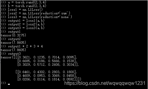

发布日期:2021-09-16 07:32:00
浏览次数:1
分类:技术文章
本文共 3290 字,大约阅读时间需要 10 分钟。
目录
Loss总结
L1Loss
mean absolute error
默认reduction参数为mean,是对所有的元素进行平均。 MSELoss

NLLLoss
negative log likelihood loss,用于多分类问题


- 输入
- x: size = (batch,class,* ), x储存每个类的log-probabilities,在神经网络添加LogSoftmax层
- y:size = (batch,* )
- 参数
- weight:1D Tensor,每个类的weight
- ignore_index:忽略类的index
- reduction:'mean’和‘sum’是标量,对所有元素进行mean或者sum
CrossEntropyLoss
结合了LogSoftmax和NLLLoss
输入和NLLLoss一样,参数也相同。
BCELoss
Binary Cross Entropy
- 输入
- x:size = (N,*),由于是2分类问题,所以没有类的信息,神经网络的最后一层应是Sigmoid,将x归入[0,1]
- y:size = (N,*),元素非0即1
- 参数
- reduction
- weight:下面代码实验weight的选取
import torch.nn as nnimport torchm = nn.Sigmoid()input = torch.randn(4, 5, requires_grad=True)target = torch.empty(4, 5).random_(2)input = m(input)loss1 = nn.BCELoss(reduction='none')output1 = loss1(input, target)print("output1:\n", output1)#w2 = torch.empty(4).random_(2)#loss2 = nn.BCELoss(reduction='none', weight=w2)#output2 = loss2(input, target)#print(w2, output2)w3 = torch.empty(4, 1).random_(2)loss3 = nn.BCELoss(reduction='none', weight=w3)output3 = loss3(input, target)print("w3:\n", w3, "\noutput3:\n", output3)w4 = torch.empty(5).random_(2)loss4 = nn.BCELoss(reduction='none', weight=w4)output4 = loss4(input, target)print("w4:\n", w4, "\noutput4:\n", output4)w5 = torch.empty(1, 5).random_(2)loss5 = nn.BCELoss(reduction='none', weight=w5)output5 = loss5(input, target)print("w5:\n", w5, "\noutput5:\n", output5)w6 = torch.empty(4, 5).random_(2)loss6 = nn.BCELoss(reduction='none', weight=w6)output6 = loss6(input, target)print("w6:\n", w6, "\noutput6:\n", output6) 结果:
output1: tensor([[1.2874, 1.0905, 2.1070, 0.3826, 2.0119], [0.3760, 0.3198, 1.0668, 0.8324, 1.1959], [1.1589, 0.7380, 0.7686, 0.7132, 0.5279], [1.0708, 1.2377, 0.3109, 0.8353, 0.4442]], grad_fn=)w3: tensor([[0.], [0.], [1.], [1.]]) output3: tensor([[0.0000, 0.0000, 0.0000, 0.0000, 0.0000], [0.0000, 0.0000, 0.0000, 0.0000, 0.0000], [1.1589, 0.7380, 0.7686, 0.7132, 0.5279], [1.0708, 1.2377, 0.3109, 0.8353, 0.4442]], grad_fn= )w4: tensor([1., 1., 0., 0., 0.]) output4: tensor([[1.2874, 1.0905, 0.0000, 0.0000, 0.0000], [0.3760, 0.3198, 0.0000, 0.0000, 0.0000], [1.1589, 0.7380, 0.0000, 0.0000, 0.0000], [1.0708, 1.2377, 0.0000, 0.0000, 0.0000]], grad_fn= )w5: tensor([[1., 1., 1., 0., 1.]]) output5: tensor([[1.2874, 1.0905, 2.1070, 0.0000, 2.0119], [0.3760, 0.3198, 1.0668, 0.0000, 1.1959], [1.1589, 0.7380, 0.7686, 0.0000, 0.5279], [1.0708, 1.2377, 0.3109, 0.0000, 0.4442]], grad_fn= )w6: tensor([[0., 1., 1., 1., 0.], [1., 0., 0., 1., 0.], [0., 1., 0., 1., 0.], [0., 1., 1., 0., 1.]]) output6: tensor([[0.0000, 1.0905, 2.1070, 0.3826, 0.0000], [0.3760, 0.0000, 0.0000, 0.8324, 0.0000], [0.0000, 0.7380, 0.0000, 0.7132, 0.0000], [0.0000, 1.2377, 0.3109, 0.0000, 0.4442]], grad_fn= )
在代码中被注释的部分报错,结果说明,BECLoss的weight是可以对每个元素设置的。
BCEWithLogitsLoss
将sigmoid与BCELoss结合在一起,比两者单独使用更具有数值稳定性。其他一样
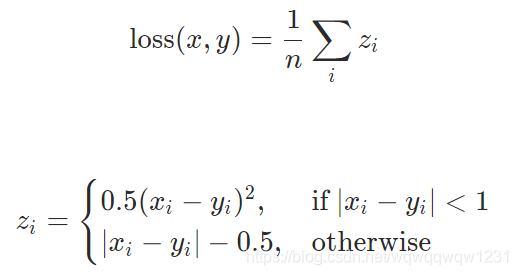
SmoothL1Loss
计算方式有差别外,其他与L1Loss没差别。
如果元素级的error低于1,则使用平方,否则使用L1。它对异常值的敏感度低于MSELoss,并且在某些情况下可以防止梯度爆炸。 转载地址:https://blog.csdn.net/wqwqqwqw1231/article/details/91627894 如侵犯您的版权,请留言回复原文章的地址,我们会给您删除此文章,给您带来不便请您谅解!
发表评论
最新留言
做的很好,不错不错
[***.243.131.199]2024年04月16日 18时16分22秒
关于作者

喝酒易醉,品茶养心,人生如梦,品茶悟道,何以解忧?唯有杜康!
-- 愿君每日到此一游!
推荐文章
pycharm的安装卸载,激活与远程调试
2019-04-26
CGAN,条件GAN
2019-04-26
改进算法1
2019-04-26
用tensorflow,pytorch框架使用GPU,指定GPU问题
2019-04-26
数据处理中ToTensor紧接着Normalize
2019-04-26
WGAN
2019-04-26
调解算法参数2
2019-04-26
调节学习率的不同策略
2019-04-26
np.ascontiguousarray(array)
2019-04-26
from scipy import misc 读取和保存图片
2019-04-26
关于Batch Normalization
2019-04-26
关于PGGAN
2019-04-26
后台挂起,让服务器运行,客户端崩溃也可以继续运行
2019-04-26
SQL中的token含义
2019-04-26
网络的权重初始化示例
2019-04-26
白红宇的个人博客 - 记录点点滴滴的事 - 您是第 306152349 位访客
访问时间: 2024-04-19 08:54:46
访问IP: 18.226.222.12
Copyright © 2020 - 2023 blog.css8.cn 京ICP备2021015314号-1
手机版