At the moment there is a wonderful course running at Standford University, called, held by Andrej Karpathy, Justin Johnson and Fei-Fei Li. Fortunately all the is provided for free and all the lectures are recorded and uploaded on. This class gives a wonderful intro to machine learning/deep learning coming along with programming assignments.

Batch Normalization

One Topic, which kept me quite busy for some time was the implementation of , especially the backward pass. Batch Normalization is a technique to provide any layer in a Neural Network with inputs that are zero mean/unit variance - and this is basically what they like! But BatchNorm consists of one more step which makes this algorithm really powerful. Let’s take a look at the BatchNorm Algorithm:

Algorithm of Batch Normalization copied from the Paper by Ioffe and Szegedy mentioned above.

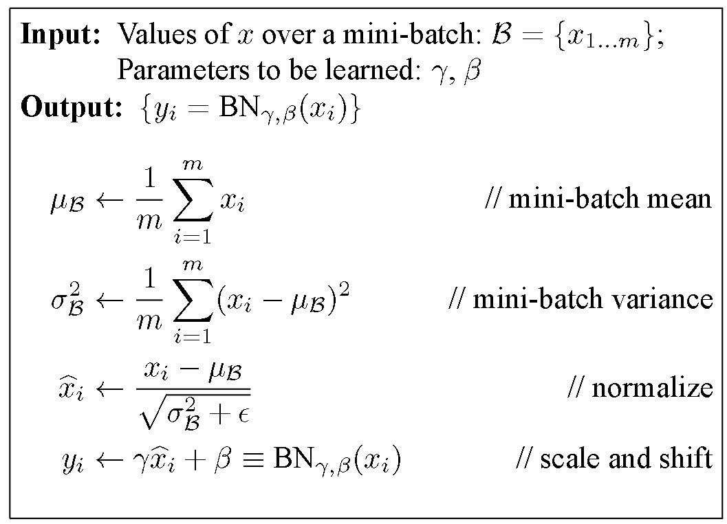
Look at the last line of the algorithm. After normalizing the input x the result is squashed through a linear function with parameters gamma and beta. These are learnable parameters of the BatchNorm Layer and make it basically possible to say “Hey!! I don’t want zero mean/unit variance input, give me back the raw input - it’s better for me.” Ifgamma = sqrt(var(x)) and beta = mean(x), the original activation is restored. This is, what makes BatchNorm really powerful. We initialize the BatchNorm Parameters to transform the input to zero mean/unit variance distributions but during training they can learn that any other distribution might be better.Anyway, I don’t want to spend to much time on explaining Batch Normalization. If you want to learn more about it, the is very well written and Andrej is explaining BatchNorm in class.

Btw: it’s called “Batch” Normalization because we perform this transformation and calculate the statistics only for a subpart (a batch) of the entire trainingsset.

Backpropagation

In this blog post I don’t want to give a lecture in Backpropagation and Stochastic Gradient Descent (SGD). For now I will assume that whoever will read this post, has some basic understanding of these principles. For the rest, let me quote Wiki:

Backpropagation, an abbreviation for “backward propagation of errors”, is a common method of training artificial neural networks used in conjunction with an optimization method such as gradient descent. The method calculates the gradient of a loss function with respect to all the weights in the network. The gradient is fed to the optimization method which in turn uses it to update the weights, in an attempt to minimize the loss function.

Uff, sounds tough, eh? I will maybe write another post about this topic but for now I want to focus on the concrete example of the backwardpass through the BatchNorm-Layer.

Computational Graph of Batch Normalization Layer

I think one of the things I learned from the cs231n class that helped me most understanding backpropagation was the explanation through computational graphs. These Graphs are a good way to visualize the computational flow of fairly complex functions by small, piecewise differentiable subfunctions. For the BatchNorm-Layer it would look something like this:

Computational graph of the BatchNorm-Layer. From left to right, following the black arrows flows the forward pass. The inputs are a matrix X and gamma and beta as vectors. From right to left, following the red arrows flows the backward pass which distributes the gradient from above layer to gamma and beta and all the way back to the input.

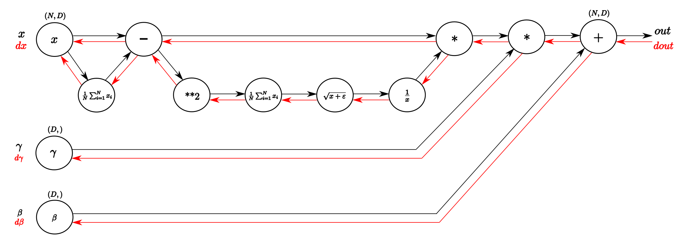
I think for all, who followed the course or who know the technique the forwardpass (black arrows) is easy and straightforward to read. From inputx we calculate the mean of every dimension in the feature space and then subtract this vector of mean values from every training example. With this done, following the lower branch, we calculate the per-dimension variance and with that the entire denominator of the normalization equation. Next we invert it and multiply it with difference of inputs and means and we havex_normalized. The last two blobs on the right perform the squashing by multiplying with the inputgamma and finally addingbeta. Et voilà, we have our Batch-Normalized output.

A vanilla implementation of the forwardpass might look like this:

def batchnorm_forward(x, gamma, beta, eps):  N, D = x.shape  #step1: calculate mean  mu = 1./N * np.sum(x, axis = 0)  #step2: subtract mean vector of every trainings example  xmu = x - mu  #step3: following the lower branch - calculation denominator  sq = xmu ** 2  #step4: calculate variance  var = 1./N * np.sum(sq, axis = 0)  #step5: add eps for numerical stability, then sqrt  sqrtvar = np.sqrt(var + eps)  #step6: invert sqrtwar  ivar = 1./sqrtvar  #step7: execute normalization  xhat = xmu * ivar  #step8: Nor the two transformation steps  gammax = gamma * xhat  #step9  out = gammax + beta  #store intermediate  cache = (xhat,gamma,xmu,ivar,sqrtvar,var,eps)  return out, cache

Note that for the exercise of the cs231n class we had to do a little more (calculate running mean and variance as well as implement different forward pass for trainings mode and test mode) but for the explanation of the backwardpass this piece of code will work.In the cache variable we store some stuff that we need for the computing of the backwardpass, as you will see now!

The power of Chain Rule for backpropagation

For all who kept on reading until now (congratulations!!), we are close to arrive at the backward pass of the BatchNorm-Layer.To fully understand the channeling of the gradient backwards through the BatchNorm-Layer you should have some basic understanding of what the is. As a little refresh follows one figure that exemplifies the use of chain rule for the backward pass in computational graphs.

The forwardpass on the left in calculates `z` as a function `f(x,y)` using the input variables `x` and `y` (This could literally be any function, examples are shown in the BatchNorm-Graph above). The right side of the figures shows the backwardpass. Receiving `dL/dz`, the gradient of the loss function with respect to `z` from above, the gradients of `x` and `y` on the loss function can be calculate by applying the chain rule, as shown in the figure.

So again, we only have to multiply the local gradient of the function with the gradient of above to channel the gradient backwards. Some derivations of some basic functions are listed in the. If you understand that, and with some more basic knowledge in calculus, what will follow is a piece of cake!

Finally: The Backpass of the Batch Normalization

In the comments of aboves code snippet I already numbered the computational steps by consecutive numbers. The Backpropagation follows these steps in reverse order, as we are literally backpassing through the computational graph. We will know take a more detailed look at every single computation of the backwardpass and by that deriving step by step a naive algorithm for the backward pass.

Step 9

Backwardpass through the last summation gate of the BatchNorm-Layer. Enclosed in brackets I put the dimensions of Input/Output

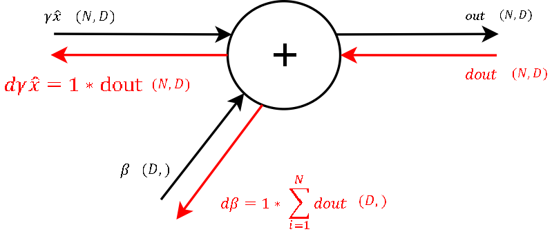
Recall that the derivation of a function f = x + y with respect to any of these two variables is1. This means to channel a gradient through a summation gate, we only need to multiply by1. And because the summation of beta during the forward pass is a row-wise summation, during the backward pass we need to sum up the gradient over all of its columns (take a look at the dimensions). So after the first step of backpropagation we already got the gradient for one learnable parameter: beta

Step 8

Next follows the backward pass through the multiplication gate of the normalized input and the vector of gamma.

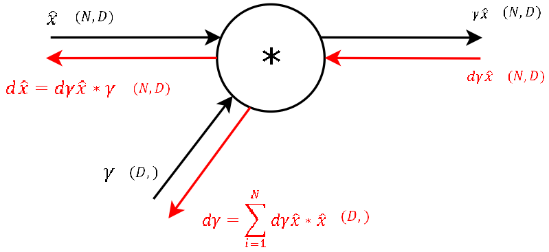
For any function f = x * y the derivation with respect to one of the inputs is simply just the other input variable. This also means, that for this step of the backward pass we need the variables used in the forward pass of this gate (luckily stored in the cache of aboves function). So again we get the gradients of the two inputs of these gates by applying chain rule ( = multiplying the local gradient with the gradient from above). For gamma, as for beta in step 9, we need to sum up the gradients over dimension N, because the multiplication was again row-wise. So we now have the gradient for the second learnable parameter of the BatchNorm-Layergamma and “only” need to backprop the gradient to the inputx, so that we then can backpropagate the gradient to any layer further downwards.

Step 7

This step during the forward pass was the final step of the normalization combining the two branches (nominator and denominator) of the computational graph. During the backward pass we will calculate the gradients that will flow separately through these two branches backwards.

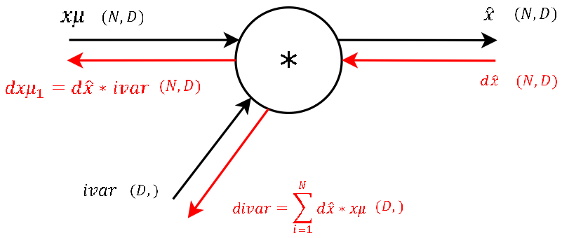
It’s basically the exact same operation, so lets not waste much time and continue. The two needed variablesxmu andivar for this step are also storedcache variable we pass to the backprop function. (And again: This is one of the main advantages of computational graphs. Splitting complex functions into a handful of simple basic operations. And like this you have a lot of repetitions!)

Step 6

This is a "one input-one output" node where, during the forward pass, we inverted the input (square root of the variance).

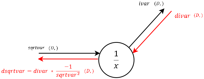
The local gradient is visualized in the image and should not be hard to derive by hand. Multiplied by the gradient from above is what we channel to the next step.sqrtvar is also one of the variables passed incache.

Step 5

Again "one input-one output". This node calculates during the forward pass the denominator of the normalization.

The derivation of the local gradient is little magic and should need no explanation.var andeps are also passed in thecache. No more words to lose!

Step 4

Also a "one input-one output" node. During the forward pass the output of this node is the variance of each feature `d for d in [1...D]`.

The derivation of this steps local gradient might look unclear at the very first glance. But it’s not that hard at the end. Let’s recall that a normal summation gate (see step 9) during the backward pass only transfers the gradient unchanged and evenly to the inputs. With that in mind, it should not be that hard to conclude, that a column-wise summation during the forward pass, during the backward pass means that we evenly distribute the gradient over all rows for each column. And not much more is done here. We create a matrix of ones with the same shape as the input sq of the forward pass, divide it element-wise by the number of rows (thats the local gradient) and multiply it by the gradient from above.

Step 3

This node outputs the square of its input, which during the forward pass was a matrix containing the input `x` subtracted by the per-feature `mean`.

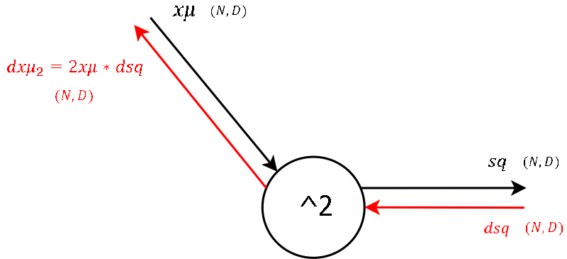
I think for all who followed until here, there is not much to explain for the derivation of the local gradient.

Step 2

Now this looks like a more fun gate! two inputs-two outputs! This node subtracts the per-feature mean row-wise of each trainings example `n for n in [1...N]` during the forward pass.

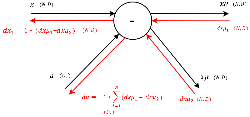
Okay lets see. One of the definitions of backprogatation and computational graphs is, that whenever we have two gradients coming to one node, we simply add them up. Knowing this, the rest is little magic as the local gradient for a subtraction is as hard to derive as for a summation. Note that for mu we have to sum up the gradients over the dimensionN (as we did before forgamma and beta).

Step 1

The function of this node is exactly the same as of step 4. Only that during the forward pass the input was `x` - the input to the BatchNorm-Layer and the output here is `mu`, a vector that contains the mean of each feature.

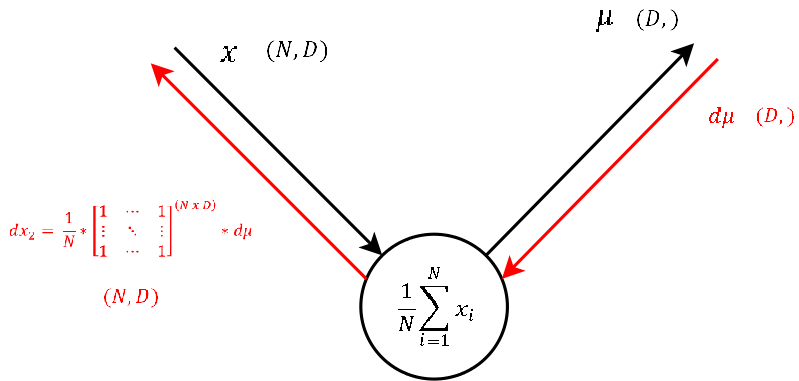
As this node executes the exact same operation as the one explained in step 4, also the backpropagation of the gradient looks the same. So let’s continue to the last step.

Step 0 - Arriving at the Input

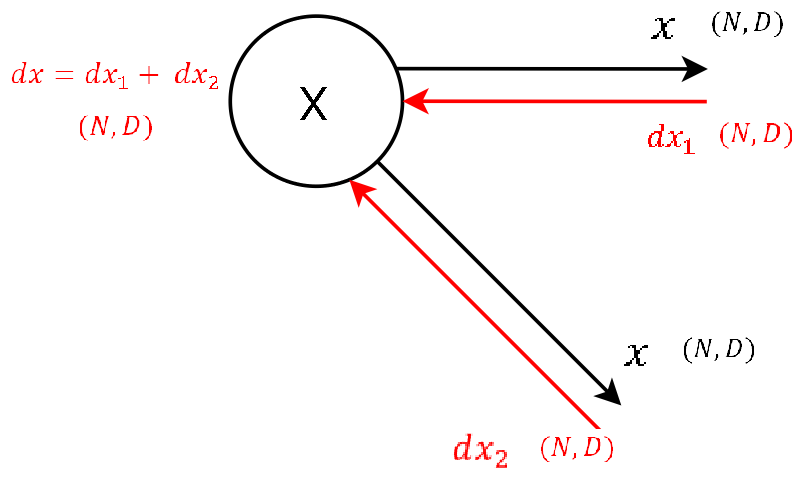
I only added this image to again visualize that at the very end we need to sum up the gradientsdx1 anddx2 to get the final gradientdx. This matrix contains the gradient of the loss function with respect to the input of the BatchNorm-Layer. This gradientdx is also what we give as input to the backwardpass of the next layer, as for this layer we receivedout from the layer above.

Naive implemantation of the backward pass through the BatchNorm-Layer

Putting together every single step the naive implementation of the backwardpass might look something like this:

def batchnorm_backward(dout, cache):  #unfold the variables stored in cache  xhat,gamma,xmu,ivar,sqrtvar,var,eps = cache  #get the dimensions of the input/output  N,D = dout.shape  #step9  dbeta = np.sum(dout, axis=0)  dgammax = dout #not necessary, but more understandable  #step8  dgamma = np.sum(dgammax*xhat, axis=0)  dxhat = dgammax * gamma  #step7  divar = np.sum(dxhat*xmu, axis=0)  dxmu1 = dxhat * ivar  #step6  dsqrtvar = -1. /(sqrtvar**2) * divar  #step5  dvar = 0.5 * 1. /np.sqrt(var+eps) * dsqrtvar  #step4  dsq = 1. /N * np.ones((N,D)) * dvar  #step3  dxmu2 = 2 * xmu * dsq  #step2  dx1 = (dxmu1 + dxmu2)  dmu = -1 * np.sum(dxmu1+dxmu2, axis=0)  #step1  dx2 = 1. /N * np.ones((N,D)) * dmu  #step0  dx = dx1 + dx2  return dx, dgamma, dbeta

Note: This is the naive implementation of the backward pass. There exists an alternative implementation, which is even a bit faster, but I personally found the naive implementation way better for the purpose of understanding backpropagation through the BatchNorm-Layer. gives a more detailed derivation of the alternative (faster) implementation. However, there is a much more calculus involved. But once you have understood the naive implementation, it might not be to hard to follow.

Some final words

First of all I would like to thank the team of the cs231n class, that gratefully make all the material freely available. This gives people like me the possibility to take part in high class courses and learn a lot about deep learning in self-study.(Secondly it made me motivated to write my first blog post!)

And as we have already passed the deadline for the second assignment, I might upload my code during the next days on github.

, the common layer structure with batch normlooks like

1. Affine transformation

   h=XW+b

where h

• ).

  where γ

  and β

  are learnable parameters and

  h^=(h−μ)(σ2+ϵ)−1/2

  contains the zero mean and unit variance version of h

  (size (N,H) ). Indeed, the parameter μ ( H ) and σ2 ( H ) are the respective average and standard deviation of each activation over the full batch (of size N ). Note that, this expression implicitly assume broadcasting as h is of size (N,H) and both μ and σ have size equal to (H)

  . A more correct expression would be

  hkl^=(hkl−μl)(σ2l+ϵ)−1/2

  where

  μl=1N∑phpl
  σ2l=1N∑p(hpl−μl)2.

  with k=1,…,N

  and l=1,…,H

  which now see a zero mean and unit variance input and where a

  contains the activations of size (N,H) . Also note that, as γ and β are learnable parameters, the network can unlearn the batch normalization transformation. In particular, the claim that the non-linearity sees a zero mean and unit variance input is only certainly true in the first forward call as γ and β are usually initialized to 1 and 0
  3. respectively.

  Derivation

  Implementing the forward pass of the batch norm transformation is straightforward

  # Forward pass mu = 1/N*np.sum(h,axis =0) # Size (H,) sigma2 = 1/N*np.sum((h-mu)**2,axis=0)# Size (H,) hath = (h-mu)*(sigma2+epsilon)**(-1./2.)y = gamma*hath+beta

  The trickypart comes with the backward pass. As the assignment proposes, thereare two strategies to implement it.

  1. Write out a computation graph composed of simple operations andbackprop through all intermediate values
  2. Work out the derivatives on paper.

  The 2nd step made me realize I did not fully understand backprogationbefore this assignment. Backpropation, an abbreviation for “backwardpropagation of errors”, calculates the gradient of a loss function L

  with respect to all the parameters of the network. In our case,we need to calculate the gradient with respect to γ , β and the input h

  .

  Mathematically, this reads dLdγ,dLdβ,dLdh

  where eachgradient with respect to a quantity contains a vector of size equal tothe quantity itself. For me, the aha-moment came when I decided toproperly write the expression for these gradients. For instance, thegradient with respect to the input h

  literally reads

  dLdh=⎛⎝⎜⎜⎜dLdh11..dLdhN1..dLdhkl...dLdh1H..dLdhNH⎞⎠⎟⎟⎟.

  To derive a close form expression for this expression, we first haveto recall that the main idea behind backpropagation is chainrule. Indeed, thanks to the previous backward pass, i.e. into ReLu inour example, we already know

  dLdy=⎛⎝⎜⎜⎜dLdy11...dLdyN1...dLdykl...dLdy1H...dLdyNH⎞⎠⎟⎟⎟.

  where

  ykl=γlh^kl+βl

  .

  We can therefore chain the gradient of the loss with respect to theinput hij

  by the gradient of the loss with respect to ALLthe outputs ykl

  which reads

  dLdhij=∑k,ldLdykldykldhij,

  which we can also chain by the gradient with respect to thecentred input h^kl

  to break down the problem a little more

  dLdhij=∑k,ldLdykldykldh^kldh^kldhij.

  The second term in the sum simply reads dykldh^kl=γl

  . All the fun part actuallycomes when looking at the third term in the sum.

  Instead of jumping right into the full derivation, let’s focus on justthe translation for one moment. Assuming the batch norm as just beinga translation, we have

  hkl^=hkl−μl

  where the expression of μl

  is given above. In that case, we have

  dh^kldhij=δi,kδj,l−1Nδj,l.

  where δi,j=1

  if i=j and 0 otherwise. Therefore, thefirst term is 1 only if k=i and l=j and the second term is 1/N only when l=j . Indeed, the gradient of h^ with respect to the j input of the i batch, which is precisely what the left hand termmeans, is non-zero only for terms in the j

  dimension. I think if youget this one, you are good to backprop whatever function youencounter so make sure you understand it before going further.

  This is just the case of translation though. What if we consider the realbatch normalization transformation ?

  In that case, the transformation considers both translation andrescaling and reads

  hkl^=(hkl−μl)(σ2l+ϵ)−1/2.

  Therefore, the gradient of the centred input h^kl

  with respect tothe input hij

  reads

  dh^kldhij=(δikδjl−1Nδjl)(σ2l+ϵ)−1/2−12(hkl−μl)dσ2ldhij(σ2l+ϵ)−3/2

  where

  σ2l=1N∑p(hpl−μl)2.

  As the gradient of the standard deviation σ2l

  with respect tothe input hij

  reads

  dσ2ldhij====1N∑p2(δipδjl−1Nδjl)(hpl−μl)2N(hil−μl)δjl−2N2∑pδjl(hpl−μl)2N(hil−μl)δjl−2Nδjl(1N∑phpl−μl)2N(hil−μl)δjl

  we finally have

  dh^kldhij=(δikδjl−1Nδjl)(σ2l+ϵ)−1/2−1N(hkl−μl)(hil−μl)δjl(σ2l+ϵ)−3/2.

  Wrapping everything together, we finally find that the gradient of theloss function L

  with respect to the layer inputs finally reads

  dLdhij=====∑kldLdykldykldh^kldh^kldhij∑kldLdyklγl((δikδjl−1Nδjl)(σ2l+ϵ)−1/2−1N(hkl−μl)(hil−μl)δjl(σ2l+ϵ)−3/2)∑kldLdyklγl((δikδjl−1Nδjl)(σ2l+ϵ)−1/2)−∑kldLdyklγl(1N(hkl−μl)(hil−μl)δjl(σ2l+ϵ)−3/2)dLdyijγj(σ2j+ϵ)−1/2−1N∑kdLdykjγj(σ2j+ϵ)−1/2−1N∑kdLdykjγj((hkj−μj)(hij−μj)(σ2j+ϵ)−3/2)1Nγj(σ2j+ϵ)−1/2(NdLdyij−∑kdLdykj−(hij−μj)(σ2j+ϵ)−1∑kdLdykj(hkj−μj))

  The gradients of the loss with respect to γ

  and β

  is muchmore straightforward and should not pose any problem if you understoodthe previous derivation. They read

  dLdγj===∑kldLdykldykldγj∑kldLdyklh^klδlj∑kdLdykj(hkj−μj)(σ2j+ϵ)−1/2
  dLdβj===∑kldLdykldykldβj∑kldLdyklδlj∑kdLdykj

  After the hard work derivation are done, you can simply just drop theseexpressions into python for the calculation. The implementation of thebatch norm backward pass looks like

  mu = 1./N*np.sum(h, axis = 0)var = 1./N*np.sum((h-mu)**2, axis = 0)dbeta = np.sum(dy, axis=0)dgamma = np.sum((h - mu) * (var + eps)**(-1. / 2.) * dy, axis=0)dh = (1. / N) * gamma * (var + eps)**(-1. / 2.) * (N * dy - np.sum(dy, axis=0)    - (h - mu) * (var + eps)**(-1.0) * np.sum(dy * (h - mu), axis=0))

  and with that, you good to go !

  Conclusion

  In this post, I focus on deriving an analytical expression for thebackward pass to implement batch-norm in a fully connected neuralnetworks. Indeed, trying to get an expression by just looking at thecentered inputs and trying to match the dimensions to get dγ

  , dβ and dh
  simply do not work this time. In contrast, workingthe derivative on papers nicely leads to the solution ;)

  To finish, I’d like to thank all the team from the CS231 Stanfordclass who do a fantastic work in vulgarizing the knowledge behindneural networks.

  For those who want to take a look to my full implementation of batchnormalization for a fully-connected neural networks, you can found it.

  Written on January 28, 2016

• Batch normalization transform

  y=γh^+β

• .

• Non-linearity activation, say ReLu for our example

  a=ReLu(y)