python 数据科学 - 【分类模型】 ☞ 稳健滴 SVM 支持向量机
 SVM Kernels
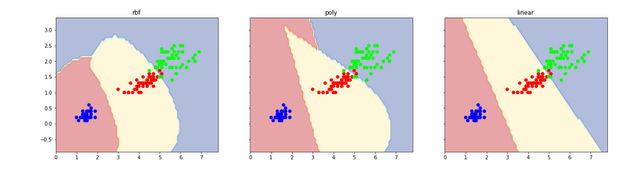
发布日期:2021-06-30 19:51:23
浏览次数:2
分类:技术文章
本文共 2446 字,大约阅读时间需要 8 分钟。
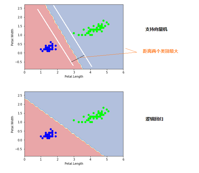
from sklearn.datasets import load_irisfrom sklearn.svm import SVCfrom sklearn.linear_model import LogisticRegressioniris = load_iris()X = iris.data[0:100,[2,3]]Y = iris.target[0:100]'''支持向量机:分界线距离两个类别的边界最远'''clf1 = SVC(kernel="linear")clf1.fit(X, Y)clf2 = LogisticRegression()clf2.fit(X, Y)from itertools import productimport numpy as npimport matplotlib.pyplot as pltdef plot_estimator(estimator, X, Y): x0_min, x0_max = X[:, 0].min() - 1, X[:, 0].max() + 1 x1_min, x1_max = X[:, 1].min() - 1, X[:, 1].max() + 1 xx, yy = np.meshgrid(np.arange(x0_min, x0_max, 0.1), np.arange(x1_min, x1_max, 0.1)) Z = estimator.predict(np.c_[xx.ravel(), yy.ravel()]) Z = Z.reshape(xx.shape) plt.plot() plt.contourf(xx, yy, Z, alpha=0.4, cmap = plt.cm.RdYlBu) plt.scatter(X[:, 0], X[:, 1], c=Y, cmap = plt.cm.brg) plt.xlabel('Petal.Length') plt.ylabel('Petal.Width') plt.show() plot_estimator(clf1, X, Y)plot_estimator(clf2, X, Y)
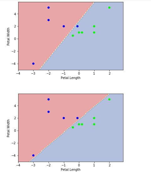
'''C, 对错误(边界的某些点)的容忍度,C值越大越不能容忍,宽度越小。C值越小间隔宽度越大。'''data = np.array([[-1,2,0],[-2,3,0],[-2,5,0],[-3,-4,0],[-0.1,2,0],[0.2,1,1],[0,1,1],[1,2,1], [1,1,1], [-0.4,0.5,1],[2,5,1]])X = data[:, :2] Y = data[:,2]# Large Marginclf = SVC(C=1.0, kernel='linear')clf.fit(X, Y)plot_estimator(clf,X,Y)# Narrow Marginclf = SVC(C=100000, kernel='linear')clf.fit(X, Y)plot_estimator(clf,X,Y)
SVM Kernels from itertools import productimport numpy as npimport matplotlib.pyplot as pltfrom sklearn.datasets import load_irisfrom sklearn.svm import SVC'''rbf,不规则线poly,弧线linear,直线(非线性数据不好使用)'''iris = load_iris()X = iris.data[:,[2,3]]Y = iris.targetclf1 = SVC(kernel="rbf")clf1.fit(X, Y)clf2 = SVC(kernel="poly")clf2.fit(X, Y)clf3 = SVC(kernel="linear")clf3.fit(X, Y)def plot_estimator(estimator, X, Y, idx, title): x0_min, x0_max = X[:, 0].min() - 1, X[:, 0].max() + 1 x1_min, x1_max = X[:, 1].min() - 1, X[:, 1].max() + 1 xx, yy = np.meshgrid(np.arange(x0_min, x0_max, 0.1), np.arange(x1_min, x1_max, 0.1)) Z = estimator.predict(np.c_[xx.ravel(), yy.ravel()]) Z = Z.reshape(xx.shape) axarr[idx].contourf(xx, yy, Z, alpha=0.4, cmap = plt.cm.RdYlBu) axarr[idx].scatter(X[:, 0], X[:, 1], c=Y, cmap = plt.cm.brg) axarr[idx].set_title(title) f, axarr = plt.subplots(1, 3, sharex='col', sharey='row', figsize=(20, 5))for idx, clf, title in zip([0,1,2],[clf1, clf2, clf3], ['rbf', 'poly', 'linear']): plot_estimator(clf, X, Y, idx, title)plt.show()
转载地址:https://lipenglin.blog.csdn.net/article/details/78083264 如侵犯您的版权,请留言回复原文章的地址,我们会给您删除此文章,给您带来不便请您谅解!
发表评论
最新留言
关注你微信了!
[***.104.42.241]2024年04月07日 10时24分35秒
关于作者

喝酒易醉,品茶养心,人生如梦,品茶悟道,何以解忧?唯有杜康!
-- 愿君每日到此一游!
推荐文章
攻防世界web进阶区easytornado详解
2019-04-30
攻防世界web进阶区web2详解
2019-04-30
xss-labs详解(上)1-10
2019-04-30
xss-labs详解(下)11-20
2019-04-30
攻防世界web进阶区ics-05详解
2019-04-30
攻防世界web进阶区FlatScience详解
2019-04-30
攻防世界web进阶区ics-04详解
2019-04-30
攻防世界web进阶区Cat详解
2019-04-30
攻防世界web进阶区bug详解
2019-04-30
攻防世界web进阶区ics-07详解
2019-04-30
攻防世界web进阶区unfinish详解
2019-04-30
攻防世界web进阶区i-got-id-200超详解
2019-04-30
sql注入总结学习
2019-04-30
leetcode46 全排列
2019-04-30
leetcode121 买卖股票的最佳时机
2019-04-30
leetcode 122 买卖股票的最佳时机II
2019-04-30
leetcode 309 最佳买卖股票含冷冻期
2019-04-30
leetcode 714 买卖股票的最佳时机含手续费
2019-04-30
leetcode3 无重复字符的最长子串
2019-04-30
leetcode 76 最小覆盖子串
2019-04-30
白红宇的个人博客 - 记录点点滴滴的事 - 您是第 310987251 位访客
访问时间: 2024-05-05 05:07:47
访问IP: 3.17.174.239
Copyright © 2020 - 2023 blog.css8.cn 京ICP备2021015314号-1
手机版