kaggle研究生招生(上)
 看来这个也是非常出名的数据集
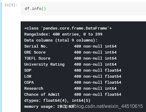
发布日期:2021-07-01 02:16:42
浏览次数:2
分类:技术文章
本文共 6187 字,大约阅读时间需要 20 分钟。
每天逛 kaggle

看来这个也是非常出名的数据集 - GRE分数(290至340)
- 托福成绩(92-120)
- 大学评级(1至5)
- 目的声明(1至5)
- 推荐信强度(1至5)
- 本科生CGPA(6.8至9.92)
- 研究经验(0或1)
- 入学率(0.34至0.97)
import pandas as pdimport matplotlib.pyplot as pltimport numpy as npimport seaborn as snsimport sysimport os
df = pd.read_csv("../input/Admission_Predict.csv",sep = ",") 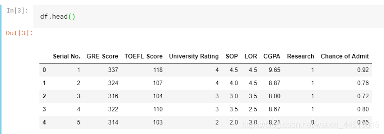
硕士入学的三个最重要特征:CGPA、GRE和托福成绩
进入硕士学位的三个最不重要的特征:研究、LOR和SOP
相关系数矩阵
fig,ax = plt.subplots(figsize=(10, 10))sns.heatmap(df.corr(), ax=ax, annot=True, linewidths=0.05, fmt= '.2f',cmap="magma")plt.show()
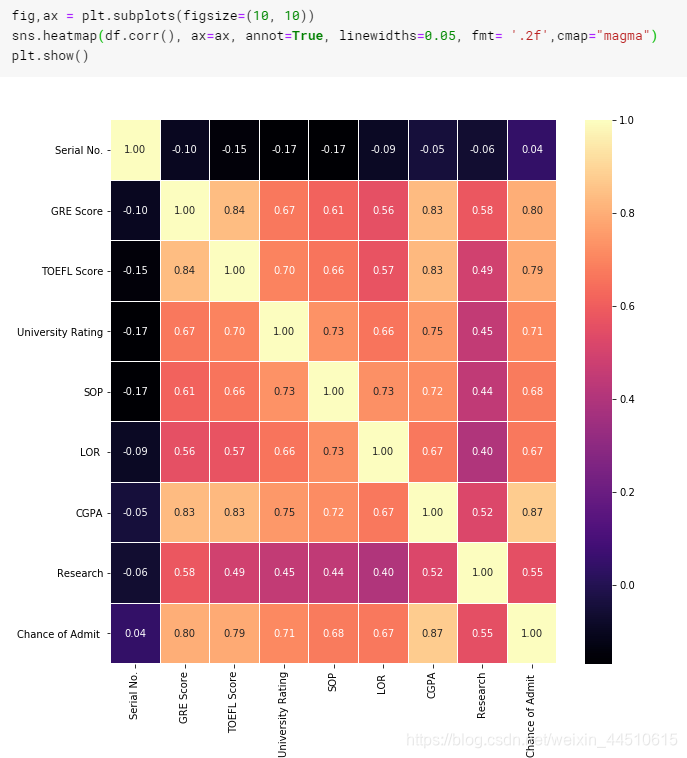
因此,本研究将成为入学机会的一个不重要的特征
print("Not Having Research:",len(df[df.Research == 0]))print("Having Research:",len(df[df.Research == 1]))y = np.array([len(df[df.Research == 0]),len(df[df.Research == 1])])x = ["Not Having Research","Having Research"]plt.bar(x,y)plt.title("Research Experience")plt.xlabel("Canditates")plt.ylabel("Frequency")plt.show() 
y = np.array([df["TOEFL Score"].min(),df["TOEFL Score"].mean(),df["TOEFL Score"].max()])x = ["Worst","Average","Best"]plt.bar(x,y)plt.title("TOEFL Scores")plt.xlabel("Level")plt.ylabel("TOEFL Score")plt.show() 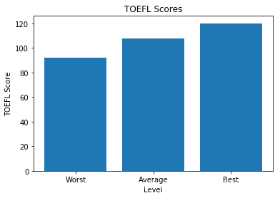
此柱状图显示GRE分数的频率。
密度介于310和330之间。在这个范围以上是候选人脱颖而出的一个很好的特征。
df["GRE Score"].plot(kind = 'hist',bins = 200,figsize = (6,6))plt.title("GRE Scores")plt.xlabel("GRE Score")plt.ylabel("Frequency")plt.show() 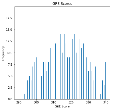
随着大学质量的提高,CGPA分数也随之提高。
plt.scatter(df["University Rating"],df.CGPA)plt.title("CGPA Scores for University Ratings")plt.xlabel("University Rating")plt.ylabel("CGPA")plt.show() 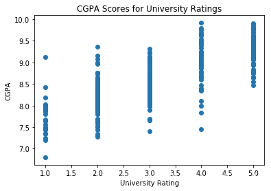
plt.scatter(df["GRE Score"],df.CGPA)plt.title("CGPA for GRE Scores")plt.xlabel("GRE Score")plt.ylabel("CGPA")plt.show() 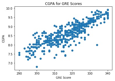
df[df.CGPA >= 8.5].plot(kind='scatter', x='GRE Score', y='TOEFL Score',color="red")plt.xlabel("GRE Score")plt.ylabel("TOEFL SCORE")plt.title("CGPA>=8.5")plt.grid(True)plt.show() 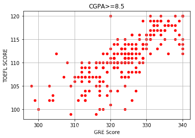
s = df[df["Chance of Admit"] >= 0.75]["University Rating"].value_counts().head(5)plt.title("University Ratings of Candidates with an 75% acceptance chance")s.plot(kind='bar',figsize=(20, 10))plt.xlabel("University Rating")plt.ylabel("Candidates")plt.show() 
plt.scatter(df["CGPA"],df.SOP)plt.xlabel("CGPA")plt.ylabel("SOP")plt.title("SOP for CGPA")plt.show() 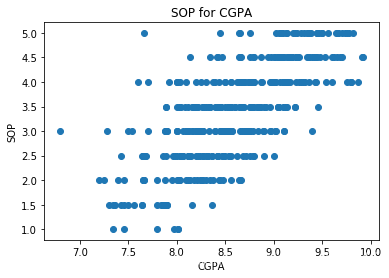
plt.scatter(df["GRE Score"],df["SOP"])plt.xlabel("GRE Score")plt.ylabel("SOP")plt.title("SOP for GRE Score")plt.show() 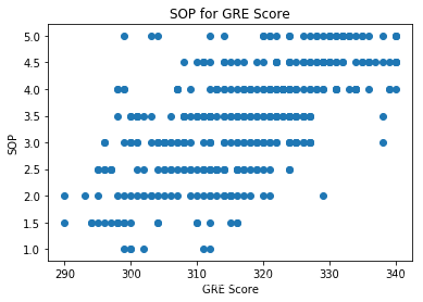
上面是数据分析过程,下面开始model的训练
去掉第一列的序号
# reading the datasetdf = pd.read_csv("../input/Admission_Predict.csv",sep = ",")# it may be needed in the future.serialNo = df["Serial No."].valuesdf.drop(["Serial No."],axis=1,inplace = True) y = df["Chance of Admit"].valuesx = df.drop(["Chance of Admit"],axis=1)# separating train (80%) and test (%20) setsfrom sklearn.model_selection import train_test_splitx_train, x_test,y_train, y_test = train_test_split(x,y,test_size = 0.20,random_state = 42)
缩放到固定范围(0-1)
# normalizationfrom sklearn.preprocessing import MinMaxScalerscalerX = MinMaxScaler(feature_range=(0, 1))x_train[x_train.columns] = scalerX.fit_transform(x_train[x_train.columns])x_test[x_test.columns] = scalerX.transform(x_test[x_test.columns])
线性模型
from sklearn.linear_model import LinearRegressionlr = LinearRegression()lr.fit(x_train,y_train)y_head_lr = lr.predict(x_test)print("real value of y_test[1]: " + str(y_test[1]) + " -> the predict: " + str(lr.predict(x_test.iloc[[1],:])))print("real value of y_test[2]: " + str(y_test[2]) + " -> the predict: " + str(lr.predict(x_test.iloc[[2],:])))from sklearn.metrics import r2_scoreprint("r_square score: ", r2_score(y_test,y_head_lr))y_head_lr_train = lr.predict(x_train)print("r_square score (train dataset): ", r2_score(y_train,y_head_lr_train)) real value of y_test[1]: 0.68 -> the predict: [0.72368741]
real value of y_test[2]: 0.9 -> the predict: [0.93536809] r_square score: 0.821208259148699 r_square score (train dataset): 0.7951946003191085随机森林
from sklearn.ensemble import RandomForestRegressorrfr = RandomForestRegressor(n_estimators = 100, random_state = 42)rfr.fit(x_train,y_train)y_head_rfr = rfr.predict(x_test) from sklearn.metrics import r2_scoreprint("r_square score: ", r2_score(y_test,y_head_rfr))print("real value of y_test[1]: " + str(y_test[1]) + " -> the predict: " + str(rfr.predict(x_test.iloc[[1],:])))print("real value of y_test[2]: " + str(y_test[2]) + " -> the predict: " + str(rfr.predict(x_test.iloc[[2],:])))y_head_rf_train = rfr.predict(x_train)print("r_square score (train dataset): ", r2_score(y_train,y_head_rf_train)) r_square score: 0.8074111823415694
real value of y_test[1]: 0.68 -> the predict: [0.7249] real value of y_test[2]: 0.9 -> the predict: [0.9407] r_square score (train dataset): 0.9634880602889714决策树
from sklearn.tree import DecisionTreeRegressordtr = DecisionTreeRegressor(random_state = 42)dtr.fit(x_train,y_train)y_head_dtr = dtr.predict(x_test) from sklearn.metrics import r2_scoreprint("r_square score: ", r2_score(y_test,y_head_dtr))print("real value of y_test[1]: " + str(y_test[1]) + " -> the predict: " + str(dtr.predict(x_test.iloc[[1],:])))print("real value of y_test[2]: " + str(y_test[2]) + " -> the predict: " + str(dtr.predict(x_test.iloc[[2],:])))y_head_dtr_train = dtr.predict(x_train)print("r_square score (train dataset): ", r2_score(y_train,y_head_dtr_train)) r_square score: 0.6262105228127393
real value of y_test[1]: 0.68 -> the predict: [0.73] real value of y_test[2]: 0.9 -> the predict: [0.94] r_square score (train dataset): 1.0线性回归和随机森林回归算法优于决策树回归算法。
y = np.array([r2_score(y_test,y_head_lr),r2_score(y_test,y_head_rfr),r2_score(y_test,y_head_dtr)])x = ["LinearRegression","RandomForestReg.","DecisionTreeReg."]plt.bar(x,y)plt.title("Comparison of Regression Algorithms")plt.xlabel("Regressor")plt.ylabel("r2_score")plt.show() 
red = plt.scatter(np.arange(0,80,5),y_head_lr[0:80:5],color = "red")green = plt.scatter(np.arange(0,80,5),y_head_rfr[0:80:5],color = "green")blue = plt.scatter(np.arange(0,80,5),y_head_dtr[0:80:5],color = "blue")black = plt.scatter(np.arange(0,80,5),y_test[0:80:5],color = "black")plt.title("Comparison of Regression Algorithms")plt.xlabel("Index of Candidate")plt.ylabel("Chance of Admit")plt.legend((red,green,blue,black),('LR', 'RFR', 'DTR', 'REAL'))plt.show() 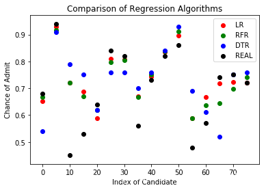
转载地址:https://maoli.blog.csdn.net/article/details/91596325 如侵犯您的版权,请留言回复原文章的地址,我们会给您删除此文章,给您带来不便请您谅解!
发表评论
最新留言
网站不错 人气很旺了 加油
[***.192.178.218]2024年04月13日 16时40分44秒
关于作者

喝酒易醉,品茶养心,人生如梦,品茶悟道,何以解忧?唯有杜康!
-- 愿君每日到此一游!
推荐文章
关于Spring MVC与前端的交互
2019-04-30
大厂经典面试题:Redis为什么这么快?
2019-04-30
Android之Retrofit基本用法篇
2019-04-30
Netty与网络协议资料整理
2019-04-30
golang实现大数据量文件的排序
2019-04-30
golang中的time包
2019-04-30
2019NOIP D4题 加工领奖
2019-04-30
2021.5.19 JS高级第二天
2019-04-30
SpringBoot内置Tomcat配置参数
2019-04-30
linux 根目录下文件夹分析
2019-04-30
linux 查看分区和文件大小
2019-04-30
Not using PCAP_FRAMES 解释(snort中)
2019-04-30
技术转管理?这些“坑”你要绕道走
2019-04-30
领域驱动设计(DDD)前夜:面向对象思想
2019-04-30
Camera驱动调试小记
2019-04-30
四线触摸屏原理
2019-04-30
C/C++如何返回一个数组/指针
2019-04-30
腾讯AI语音识别API踩坑记录
2019-04-30
YbtOJ——递推算法【例题4】传球游戏
2019-04-30
白红宇的个人博客 - 记录点点滴滴的事 - 您是第 311502810 位访客
访问时间: 2024-05-06 21:57:32
访问IP: 3.144.84.155
Copyright © 2020 - 2023 blog.css8.cn 京ICP备2021015314号-1
手机版