本文共 12120 字，大约阅读时间需要 40 分钟。

上次将数据训练了模型

由于数据中的大多数候选人都有70%以上的机会，许多不成功的候选人都没有很好的预测。

df["Chance of Admit"].plot(kind = 'hist',bins = 200,figsize = (6,6))plt.title("Chance of Admit")plt.xlabel("Chance of Admit")plt.ylabel("Frequency")plt.show()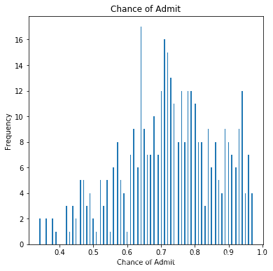

为分类准备数据

如果候选人的录取机会大于80%，则该候选人将获得1个标签。

如果候选人的录取机会小于或等于80%，则该候选人将获得0标签。

# reading the datasetdf = pd.read_csv("../input/Admission_Predict.csv",sep = ",")# it may be needed in the future.serialNo = df["Serial No."].valuesdf.drop(["Serial No."],axis=1,inplace = True)y = df["Chance of Admit"].valuesx = df.drop(["Chance of Admit"],axis=1)# separating train (80%) and test (%20) setsfrom sklearn.model_selection import train_test_splitx_train, x_test,y_train, y_test = train_test_split(x,y,test_size = 0.20,random_state = 42)# normalizationfrom sklearn.preprocessing import MinMaxScalerscalerX = MinMaxScaler(feature_range=(0, 1))x_train[x_train.columns] = scalerX.fit_transform(x_train[x_train.columns])x_test[x_test.columns] = scalerX.transform(x_test[x_test.columns])y_train_01 = [1 if each > 0.8 else 0 for each in y_train]y_test_01  = [1 if each > 0.8 else 0 for each in y_test]# list to arrayy_train_01 = np.array(y_train_01)y_test_01 = np.array(y_test_01)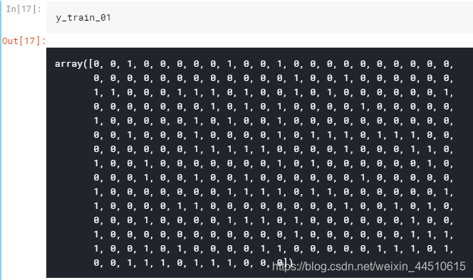

逻辑回归

from sklearn.linear_model import LogisticRegressionlrc = LogisticRegression()lrc.fit(x_train,y_train_01)print("score: ", lrc.score(x_test,y_test_01))print("real value of y_test_01[1]: " + str(y_test_01[1]) + " -> the predict: " + str(lrc.predict(x_test.iloc[[1],:])))print("real value of y_test_01[2]: " + str(y_test_01[2]) + " -> the predict: " + str(lrc.predict(x_test.iloc[[2],:])))# confusion matrixfrom sklearn.metrics import confusion_matrixcm_lrc = confusion_matrix(y_test_01,lrc.predict(x_test))# print("y_test_01 == 1 :" + str(len(y_test_01[y_test_01==1]))) # 29# cm visualizationimport seaborn as snsimport matplotlib.pyplot as pltf, ax = plt.subplots(figsize =(5,5))sns.heatmap(cm_lrc,annot = True,linewidths=0.5,linecolor="red",fmt = ".0f",ax=ax)plt.title("Test for Test Dataset")plt.xlabel("predicted y values")plt.ylabel("real y values")plt.show()from sklearn.metrics import precision_score, recall_scoreprint("precision_score: ", precision_score(y_test_01,lrc.predict(x_test)))print("recall_score: ", recall_score(y_test_01,lrc.predict(x_test)))from sklearn.metrics import f1_scoreprint("f1_score: ",f1_score(y_test_01,lrc.predict(x_test)))

score: 0.9

real value of y_test_01[1]: 0 -> the predict: [0] real value of y_test_01[2]: 1 -> the predict: [1]

precision_score: 0.9565217391304348 recall_score: 0.7586206896551724 f1_score: 0.8461538461538461

Test for Train Dataset:

cm_lrc_train = confusion_matrix(y_train_01,lrc.predict(x_train))f, ax = plt.subplots(figsize =(5,5))sns.heatmap(cm_lrc_train,annot = True,linewidths=0.5,linecolor="red",fmt = ".0f",ax=ax)plt.xlabel("predicted y values")plt.ylabel("real y values")plt.title("Test for Train Dataset")plt.show()

SVC

from sklearn.svm import SVCsvm = SVC(random_state = 1)svm.fit(x_train,y_train_01)print("score: ", svm.score(x_test,y_test_01))print("real value of y_test_01[1]: " + str(y_test_01[1]) + " -> the predict: " + str(svm.predict(x_test.iloc[[1],:])))print("real value of y_test_01[2]: " + str(y_test_01[2]) + " -> the predict: " + str(svm.predict(x_test.iloc[[2],:])))# confusion matrixfrom sklearn.metrics import confusion_matrixcm_svm = confusion_matrix(y_test_01,svm.predict(x_test))# print("y_test_01 == 1 :" + str(len(y_test_01[y_test_01==1]))) # 29# cm visualizationimport seaborn as snsimport matplotlib.pyplot as pltf, ax = plt.subplots(figsize =(5,5))sns.heatmap(cm_svm,annot = True,linewidths=0.5,linecolor="red",fmt = ".0f",ax=ax)plt.title("Test for Test Dataset")plt.xlabel("predicted y values")plt.ylabel("real y values")plt.show()from sklearn.metrics import precision_score, recall_scoreprint("precision_score: ", precision_score(y_test_01,svm.predict(x_test)))print("recall_score: ", recall_score(y_test_01,svm.predict(x_test)))from sklearn.metrics import f1_scoreprint("f1_score: ",f1_score(y_test_01,svm.predict(x_test)))

score: 0.9

real value of y_test_01[1]: 0 -> the predict: [0] real value of y_test_01[2]: 1 -> the predict: [1]

precision_score: 0.9565217391304348

recall_score: 0.7586206896551724 f1_score: 0.8461538461538461

Test for Train Dataset

cm_svm_train = confusion_matrix(y_train_01,svm.predict(x_train))f, ax = plt.subplots(figsize =(5,5))sns.heatmap(cm_svm_train,annot = True,linewidths=0.5,linecolor="red",fmt = ".0f",ax=ax)plt.xlabel("predicted y values")plt.ylabel("real y values")plt.title("Test for Train Dataset")plt.show()

朴素贝叶斯

from sklearn.naive_bayes import GaussianNBnb = GaussianNB()nb.fit(x_train,y_train_01)print("score: ", nb.score(x_test,y_test_01))print("real value of y_test_01[1]: " + str(y_test_01[1]) + " -> the predict: " + str(nb.predict(x_test.iloc[[1],:])))print("real value of y_test_01[2]: " + str(y_test_01[2]) + " -> the predict: " + str(nb.predict(x_test.iloc[[2],:])))# confusion matrixfrom sklearn.metrics import confusion_matrixcm_nb = confusion_matrix(y_test_01,nb.predict(x_test))# print("y_test_01 == 1 :" + str(len(y_test_01[y_test_01==1]))) # 29# cm visualizationimport seaborn as snsimport matplotlib.pyplot as pltf, ax = plt.subplots(figsize =(5,5))sns.heatmap(cm_nb,annot = True,linewidths=0.5,linecolor="red",fmt = ".0f",ax=ax)plt.title("Test for Test Dataset")plt.xlabel("predicted y values")plt.ylabel("real y values")plt.show()from sklearn.metrics import precision_score, recall_scoreprint("precision_score: ", precision_score(y_test_01,nb.predict(x_test)))print("recall_score: ", recall_score(y_test_01,nb.predict(x_test)))from sklearn.metrics import f1_scoreprint("f1_score: ",f1_score(y_test_01,nb.predict(x_test)))

score: 0.9625

real value of y_test_01[1]: 0 -> the predict: [0] real value of y_test_01[2]: 1 -> the predict: [1]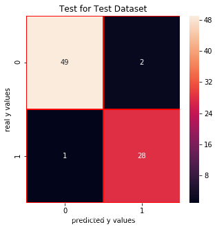

precision_score: 0.9333333333333333 recall_score: 0.9655172413793104 f1_score: 0.9491525423728815

Test for Train Dataset:

cm_nb_train = confusion_matrix(y_train_01,nb.predict(x_train))f, ax = plt.subplots(figsize =(5,5))sns.heatmap(cm_nb_train,annot = True,linewidths=0.5,linecolor="red",fmt = ".0f",ax=ax)plt.xlabel("predicted y values")plt.ylabel("real y values")plt.title("Test for Train Dataset")plt.show()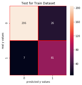

决策树

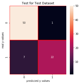
from sklearn.tree import DecisionTreeClassifierdtc = DecisionTreeClassifier()dtc.fit(x_train,y_train_01)print("score: ", dtc.score(x_test,y_test_01))print("real value of y_test_01[1]: " + str(y_test_01[1]) + " -> the predict: " + str(dtc.predict(x_test.iloc[[1],:])))print("real value of y_test_01[2]: " + str(y_test_01[2]) + " -> the predict: " + str(dtc.predict(x_test.iloc[[2],:])))# confusion matrixfrom sklearn.metrics import confusion_matrixcm_dtc = confusion_matrix(y_test_01,dtc.predict(x_test))# print("y_test_01 == 1 :" + str(len(y_test_01[y_test_01==1]))) # 29# cm visualizationimport seaborn as snsimport matplotlib.pyplot as pltf, ax = plt.subplots(figsize =(5,5))sns.heatmap(cm_dtc,annot = True,linewidths=0.5,linecolor="red",fmt = ".0f",ax=ax)plt.title("Test for Test Dataset")plt.xlabel("predicted y values")plt.ylabel("real y values")plt.show()from sklearn.metrics import precision_score, recall_scoreprint("precision_score: ", precision_score(y_test_01,dtc.predict(x_test)))print("recall_score: ", recall_score(y_test_01,dtc.predict(x_test)))from sklearn.metrics import f1_scoreprint("f1_score: ",f1_score(y_test_01,dtc.predict(x_test)))

score: 0.9375

real value of y_test_01[1]: 0 -> the predict: [0] real value of y_test_01[2]: 1 -> the predict: [1]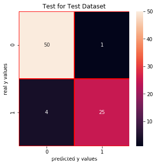

precision_score: 0.9615384615384616

recall_score: 0.8620689655172413 f1_score: 0.9090909090909091

Test for Train Dataset

cm_dtc_train = confusion_matrix(y_train_01,dtc.predict(x_train))f, ax = plt.subplots(figsize =(5,5))sns.heatmap(cm_dtc_train,annot = True,linewidths=0.5,linecolor="red",fmt = ".0f",ax=ax)plt.xlabel("predicted y values")plt.ylabel("real y values")plt.title("Test for Train Dataset")plt.show()

随机森林

from sklearn.ensemble import RandomForestClassifierrfc = RandomForestClassifier(n_estimators = 100,random_state = 1)rfc.fit(x_train,y_train_01)print("score: ", rfc.score(x_test,y_test_01))print("real value of y_test_01[1]: " + str(y_test_01[1]) + " -> the predict: " + str(rfc.predict(x_test.iloc[[1],:])))print("real value of y_test_01[2]: " + str(y_test_01[2]) + " -> the predict: " + str(rfc.predict(x_test.iloc[[2],:])))# confusion matrixfrom sklearn.metrics import confusion_matrixcm_rfc = confusion_matrix(y_test_01,rfc.predict(x_test))# print("y_test_01 == 1 :" + str(len(y_test_01[y_test_01==1]))) # 29# cm visualizationimport seaborn as snsimport matplotlib.pyplot as pltf, ax = plt.subplots(figsize =(5,5))sns.heatmap(cm_rfc,annot = True,linewidths=0.5,linecolor="red",fmt = ".0f",ax=ax)plt.title("Test for Test Dataset")plt.xlabel("predicted y values")plt.ylabel("real y values")plt.show()from sklearn.metrics import precision_score, recall_scoreprint("precision_score: ", precision_score(y_test_01,rfc.predict(x_test)))print("recall_score: ", recall_score(y_test_01,rfc.predict(x_test)))from sklearn.metrics import f1_scoreprint("f1_score: ",f1_score(y_test_01,rfc.predict(x_test)))

score: 0.9375

real value of y_test_01[1]: 0 -> the predict: [0] real value of y_test_01[2]: 1 -> the predict: [1] precision_score: 0.9615384615384616 recall_score: 0.8620689655172413 f1_score: 0.9090909090909091

Test for Train Dataset

cm_rfc_train = confusion_matrix(y_train_01,rfc.predict(x_train))f, ax = plt.subplots(figsize =(5,5))sns.heatmap(cm_rfc_train,annot = True,linewidths=0.5,linecolor="red",fmt = ".0f",ax=ax)plt.xlabel("predicted y values")plt.ylabel("real y values")plt.title("Test for Train Dataset")plt.show()

kNN

from sklearn.neighbors import KNeighborsClassifier# finding k valuescores = []for each in range(1,50):    knn_n = KNeighborsClassifier(n_neighbors = each)    knn_n.fit(x_train,y_train_01)    scores.append(knn_n.score(x_test,y_test_01))    plt.plot(range(1,50),scores)plt.xlabel("k")plt.ylabel("accuracy")plt.show()knn = KNeighborsClassifier(n_neighbors = 3) # n_neighbors = kknn.fit(x_train,y_train_01)print("score of 3 :",knn.score(x_test,y_test_01))print("real value of y_test_01[1]: " + str(y_test_01[1]) + " -> the predict: " + str(knn.predict(x_test.iloc[[1],:])))print("real value of y_test_01[2]: " + str(y_test_01[2]) + " -> the predict: " + str(knn.predict(x_test.iloc[[2],:])))# confusion matrixfrom sklearn.metrics import confusion_matrixcm_knn = confusion_matrix(y_test_01,knn.predict(x_test))# print("y_test_01 == 1 :" + str(len(y_test_01[y_test_01==1]))) # 29# cm visualizationimport seaborn as snsimport matplotlib.pyplot as pltf, ax = plt.subplots(figsize =(5,5))sns.heatmap(cm_knn,annot = True,linewidths=0.5,linecolor="red",fmt = ".0f",ax=ax)plt.title("Test for Test Dataset")plt.xlabel("predicted y values")plt.ylabel("real y values")plt.show()from sklearn.metrics import precision_score, recall_scoreprint("precision_score: ", precision_score(y_test_01,knn.predict(x_test)))print("recall_score: ", recall_score(y_test_01,knn.predict(x_test)))from sklearn.metrics import f1_scoreprint("f1_score: ",f1_score(y_test_01,knn.predict(x_test)))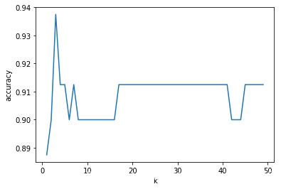

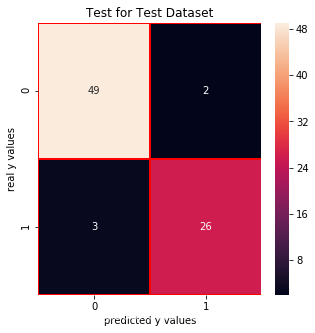
score of 3 : 0.9375 real value of y_test_01[1]: 0 -> the predict: [0] real value of y_test_01[2]: 1 -> the predict: [1]

precision_score: 0.9285714285714286 recall_score: 0.896551724137931 f1_score: 0.912280701754386

Test for Train Dataset:

cm_knn_train = confusion_matrix(y_train_01,knn.predict(x_train))f, ax = plt.subplots(figsize =(5,5))sns.heatmap(cm_knn_train,annot = True,linewidths=0.5,linecolor="red",fmt = ".0f",ax=ax)plt.xlabel("predicted y values")plt.ylabel("real y values")plt.title("Test for Train Dataset")plt.show()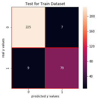

所有分类算法都取得了大约90%的成功。最成功的是高斯朴素贝叶斯，得分为96%。

y = np.array([lrc.score(x_test,y_test_01),svm.score(x_test,y_test_01),nb.score(x_test,y_test_01),dtc.score(x_test,y_test_01),rfc.score(x_test,y_test_01),knn.score(x_test,y_test_01)])#x = ["LogisticRegression","SVM","GaussianNB","DecisionTreeClassifier","RandomForestClassifier","KNeighborsClassifier"]x = ["LogisticReg.","SVM","GNB","Dec.Tree","Ran.Forest","KNN"]plt.bar(x,y)plt.title("Comparison of Classification Algorithms")plt.xlabel("Classfication")plt.ylabel("Score")plt.show()

上文是回归算法，此文分类

转载地址：https://maoli.blog.csdn.net/article/details/92020207 如侵犯您的版权，请留言回复原文章的地址，我们会给您删除此文章，给您带来不便请您谅解！