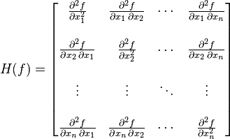
海森矩阵就是二阶偏导函数的方阵.他描述了局部的曲率函数-白红宇的个人博客

发布日期：2021-07-01 05:57:15 浏览次数：3 分类：技术文章

本文共 2581 字，大约阅读时间需要 8 分钟。

In , the Hessian matrix is the of second-order of a; that is, it describes the local curvature of a function of many variables. The Hessian matrix was developed in the 19th century by the mathematician and later named after him. Hesse himself had used the term "functional determinants".

海森矩阵就是二阶偏导函数的方阵.他描述了局部的曲率函数.

Given the -valued function

$f(x_1, x_2, \dots, x_n),\,\!$

if all second partial derivatives of f exist, then the Hessian matrix of f is the matrix

$H(f)_{ij}(x) = D_i D_j f(x)\,\!$

where x = (x₁, x₂, ..., x_n) and D_i is the differentiation operator with respect to the ith argument and the Hessian becomes

$H(f) = \begin{bmatrix} \frac{\partial^2 f}{\partial x_1^2} & \frac{\partial^2 f}{\partial x_1\,\partial x_2} & \cdots & \frac{\partial^2 f}{\partial x_1\,\partial x_n} \\ \ \frac{\partial^2 f}{\partial x_2\,\partial x_1} & \frac{\partial^2 f}{\partial x_2^2} & \cdots & \frac{\partial^2 f}{\partial x_2\,\partial x_n} \\ \ \vdots & \vdots & \ddots & \vdots \\ \ \frac{\partial^2 f}{\partial x_n\,\partial x_1} & \frac{\partial^2 f}{\partial x_n\,\partial x_2} & \cdots & \frac{\partial^2 f}{\partial x_n^2} \end{bmatrix}$

Some mathematicians define the Hessian as the of the above matrix.

Hessian matrices are used in large-scale problems within -type methods because they are the coefficient of the quadratic term of a local of a function. That is,

$y=f(\mathbf{x}+\Delta\mathbf{x})\approx f(\mathbf{x}) + J(\mathbf{x})\Delta \mathbf{x} +\frac{1}{2} \Delta\mathbf{x}^\mathrm{T} H(\mathbf{x}) \Delta\mathbf{x}$

where J is the , which is a vector (the ) for scalar-valued functions. The full Hessian matrix can be difficult to compute in practice; in such situations, algorithms have been developed that use approximations to the Hessian. The most well-known quasi-Newton algorithm is the algorithm.

在数学中，海森矩阵（Hessian matrix 或 Hessian）是一个自变量为向量的实值函数的二阶偏导数组成的方块矩阵，此函数如下：

$f(x_1, x_2, \dots, x_n),$

如果 f 所有的二阶导数都存在，那么 f 的海森矩阵即：

H(f)ij(x) = DiDjf(x)

其中 $x = (x_1, x_2, \dots, x_n)$ ，即

$H(f) = \begin{bmatrix}\frac{\partial^2 f}{\partial x_1^2} & \frac{\partial^2 f}{\partial x_1\,\partial x_2} & \cdots & \frac{\partial^2 f}{\partial x_1\,\partial x_n} \\ \\\frac{\partial^2 f}{\partial x_2\,\partial x_1} & \frac{\partial^2 f}{\partial x_2^2} & \cdots & \frac{\partial^2 f}{\partial x_2\,\partial x_n} \\ \\\vdots & \vdots & \ddots & \vdots \\ \\\frac{\partial^2 f}{\partial x_n\,\partial x_1} & \frac{\partial^2 f}{\partial x_n\,\partial x_2} & \cdots & \frac{\partial^2 f}{\partial x_n^2}\end{bmatrix}$

可见，多元函数的二阶导数就是一个海森矩阵

海森矩阵被应用于牛顿法解决的大规模优化问题。

混合偏导数和海森矩阵的对称性

海森矩阵的混合偏导数是海森矩阵非主对角线上的元素。假如他们是连续的，那么求导顺序没有区别，即

$\frac {\partial}{\partial x} \left( \frac { \partial f }{ \partial y} \right) = \frac {\partial}{\partial y} \left( \frac { \partial f }{ \partial x} \right)$

上式也可写为

$f_{xy} = f_{yx} \,$

在正式写法中，如果 f 函数在区域 D 内连续并处处存在二阶导数，那么 f的海森矩阵在 D 区域内为对称矩阵。

给定二阶导数连续的函数，海森矩阵的行列式，可用于分辨 f 的临界点是属于鞍点还是极值点。

对于 f 的临界点 (x0,y0) 一点，有 $\frac{\partial f(x_0, y_0)}{\partial x} = \frac{\partial f(x_0, y_0)}{\partial y} = 0$ ，然而凭一阶导数不能判断它是鞍点、局部极大点还是局部极小点。海森矩阵可能解答这个问题。

$H = \begin{vmatrix}\frac{\partial^2 f}{\partial x^2} & \frac{\partial^2 f}{\partial x\,\partial y} \\ \\\frac{\partial^2 f}{\partial y\,\partial x} & \frac{\partial^2 f}{\partial y^2} \end{vmatrix} = \frac{\partial^2 f}{\partial x^2} \frac{\partial^2 f}{\partial y^2} - (\frac{\partial^2 f}{\partial y\,\partial x})^2$

H > 0 ：若 $\frac{\partial^2 f}{\partial x^2} > 0$ ，则(x0,y0)是局部极小点；若 $\frac{\partial^2 f}{\partial x^2} < 0$ ，则(x0,y0)是局部极大点。

H < 0 ：(x0,y0)是鞍点。

H = 0 ：二阶导数无法判断该临界点的性质，得从更高阶的导数以泰勒公式考虑。

MATLAB中获得Hessian矩阵：

The Hessian of a scalar valued function f:Rn

首先类比一下一维。Jacobian相当于一阶导数，Hessian相当于二阶导数。一维函数的导数的motivation是很明显的。二阶导数的零点就是一阶导数的极值点。对于很多应用，我们不仅关心一阶导数的零点，也关心一阶导数的极值点，比如信号处理中，信号的一阶导数的极值点反映信号变化的最剧烈程度。极值点寻求在编程时不方便，不如找二阶导数的零点。

Jacobian对于标量函数f: Rn-> R1，实际是个向量，这个向量实际上就是函数的梯度gradient。gradient根据Cauchy-Swartz公式，指向的是在某处方向导数取极大值的方向。在二维图像处理中，可用gradient来检测灰度值的边缘。

对于向量场F: Rn-> Rm, Jacobian的每一行实际都是一个梯度。且有 F（X)=F(P)+J(P)(X-P)+O(||X-P||) 这个式子的每一行都是一个分量的局部线性化。

考虑一个二维的数字图像线性变换（Homography， image warping), 以有限差分代替微分，可作类似分析。

H: 像素（x,y)-->像素(u,v)

u=u（x,y) v=v(x,y)

则其Jacobian为

[ u'(x) u'(y)]

[ v'(x) v'(y)]

反映了局部图像的变形程度。

最理想的情况 u'(x)=1,v'(y)=1,u'(y)=0,v'(x)=0.说明图像维持原状。

由于 dudv=|det(Jacobian(x,y))|dxdy （此式的有效性可参考换元法）

[注：]有的书上称det(Jacobian(x,y)）为Jacobian.

说明面积微元改变的程度由|det(Jacobian(x,y))|决定

当|det(Jacobian(x,y))|=1时，说明面积不变，

当|det(Jacobian(x,y))|<1时，说明面积压缩，出现了像素丢失现象。

当|det(Jacobian(x,y))|>1时，说明面积扩张，需要进行像素插值。

另外，由Jacobian矩阵的特征值或奇异值，可作类似说明。可参考Wielandt-Hoffman定理

Hessian矩阵定义在标量函数上，对于矢量函数，则成为一个rank 3的张量。

转载地址：https://panda1234lee.blog.csdn.net/article/details/9472997 如侵犯您的版权，请留言回复原文章的地址，我们会给您删除此文章，给您带来不便请您谅解！

上一篇：GeoJSON格式规范

下一篇：[转载]SURF 与 SIFT的共同点与不同点

发表评论

关于作者

喝酒易醉，品茶养心，人生如梦，品茶悟道，何以解忧？唯有杜康！

-- 愿君每日到此一游！

发表评论

最新留言

关于作者

推荐文章