pytorch yolov3 代码详解_YOLOv3作者JR官方Pytorch检测代码-白红宇的个人博客

pytorch yolov3 代码详解_YOLOv3作者JR官方Pytorch检测代码

发布日期：2021-06-24 17:29:55 浏览次数：3 分类：技术文章

本文共 19523 字，大约阅读时间需要 65 分钟。

一：前言

代码链接：

ayooshkathuria/YOLO_v3_tutorial_from_scratchgithub.com

官方注释翻译：

深度智能：从零开始实现YOLO v3（Part1）zhuanlan.zhihu.com

推荐注释(来自王若霄师兄 @王若霄的工作)：

王若霄：超详细的Pytorch版yolov3代码中文注释详解（一）zhuanlan.zhihu.com

本文进行的工作：

上面已经对代码各模块进行了详细解读，此次工作是完整进行一次detect(detect.py文件).

请详细研究cfg网络层信息：https://zhuanlan.zhihu.com/p/36920744（找到配置文件）

>..> 我是真的蠢！！！tensorflow、pytorch图片的输入格式都是（H，W）

重要网络参考：

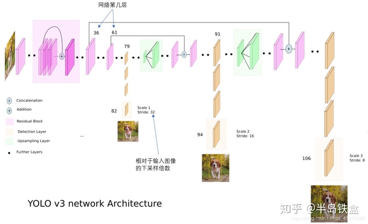
他是完整的一次检测网络，有输入输出、route、residual，注意索引index(layer)和代码的索引前后关系相同(如：route -4 ，往后索引四层，表中：83 route 79，就是往后4层到达79 ).

下面会多次使用此表！

Demolayer     filters    size              input                output    0 conv     32  3 x 3 / 1   416 x 416 x   3   ->   416 x 416 x  32  0.299 BFLOPs    1 conv     64  3 x 3 / 2   416 x 416 x  32   ->   208 x 208 x  64  1.595 BFLOPs    2 conv     32  1 x 1 / 1   208 x 208 x  64   ->   208 x 208 x  32  0.177 BFLOPs    3 conv     64  3 x 3 / 1   208 x 208 x  32   ->   208 x 208 x  64  1.595 BFLOPs    4 res    1                 208 x 208 x  64   ->   208 x 208 x  64    5 conv    128  3 x 3 / 2   208 x 208 x  64   ->   104 x 104 x 128  1.595 BFLOPs    6 conv     64  1 x 1 / 1   104 x 104 x 128   ->   104 x 104 x  64  0.177 BFLOPs    7 conv    128  3 x 3 / 1   104 x 104 x  64   ->   104 x 104 x 128  1.595 BFLOPs    8 res    5                 104 x 104 x 128   ->   104 x 104 x 128    9 conv     64  1 x 1 / 1   104 x 104 x 128   ->   104 x 104 x  64  0.177 BFLOPs   10 conv    128  3 x 3 / 1   104 x 104 x  64   ->   104 x 104 x 128  1.595 BFLOPs   11 res    8                 104 x 104 x 128   ->   104 x 104 x 128   12 conv    256  3 x 3 / 2   104 x 104 x 128   ->    52 x  52 x 256  1.595 BFLOPs   13 conv    128  1 x 1 / 1    52 x  52 x 256   ->    52 x  52 x 128  0.177 BFLOPs   14 conv    256  3 x 3 / 1    52 x  52 x 128   ->    52 x  52 x 256  1.595 BFLOPs   15 res   12                  52 x  52 x 256   ->    52 x  52 x 256   16 conv    128  1 x 1 / 1    52 x  52 x 256   ->    52 x  52 x 128  0.177 BFLOPs   17 conv    256  3 x 3 / 1    52 x  52 x 128   ->    52 x  52 x 256  1.595 BFLOPs   18 res   15                  52 x  52 x 256   ->    52 x  52 x 256   19 conv    128  1 x 1 / 1    52 x  52 x 256   ->    52 x  52 x 128  0.177 BFLOPs   20 conv    256  3 x 3 / 1    52 x  52 x 128   ->    52 x  52 x 256  1.595 BFLOPs   21 res   18                  52 x  52 x 256   ->    52 x  52 x 256   22 conv    128  1 x 1 / 1    52 x  52 x 256   ->    52 x  52 x 128  0.177 BFLOPs   23 conv    256  3 x 3 / 1    52 x  52 x 128   ->    52 x  52 x 256  1.595 BFLOPs   24 res   21                  52 x  52 x 256   ->    52 x  52 x 256   25 conv    128  1 x 1 / 1    52 x  52 x 256   ->    52 x  52 x 128  0.177 BFLOPs   26 conv    256  3 x 3 / 1    52 x  52 x 128   ->    52 x  52 x 256  1.595 BFLOPs   27 res   24                  52 x  52 x 256   ->    52 x  52 x 256   28 conv    128  1 x 1 / 1    52 x  52 x 256   ->    52 x  52 x 128  0.177 BFLOPs   29 conv    256  3 x 3 / 1    52 x  52 x 128   ->    52 x  52 x 256  1.595 BFLOPs   30 res   27                  52 x  52 x 256   ->    52 x  52 x 256   31 conv    128  1 x 1 / 1    52 x  52 x 256   ->    52 x  52 x 128  0.177 BFLOPs   32 conv    256  3 x 3 / 1    52 x  52 x 128   ->    52 x  52 x 256  1.595 BFLOPs   33 res   30                  52 x  52 x 256   ->    52 x  52 x 256   34 conv    128  1 x 1 / 1    52 x  52 x 256   ->    52 x  52 x 128  0.177 BFLOPs   35 conv    256  3 x 3 / 1    52 x  52 x 128   ->    52 x  52 x 256  1.595 BFLOPs   36 res   33                  52 x  52 x 256   ->    52 x  52 x 256   37 conv    512  3 x 3 / 2    52 x  52 x 256   ->    26 x  26 x 512  1.595 BFLOPs   38 conv    256  1 x 1 / 1    26 x  26 x 512   ->    26 x  26 x 256  0.177 BFLOPs   39 conv    512  3 x 3 / 1    26 x  26 x 256   ->    26 x  26 x 512  1.595 BFLOPs   40 res   37                  26 x  26 x 512   ->    26 x  26 x 512   41 conv    256  1 x 1 / 1    26 x  26 x 512   ->    26 x  26 x 256  0.177 BFLOPs   42 conv    512  3 x 3 / 1    26 x  26 x 256   ->    26 x  26 x 512  1.595 BFLOPs   43 res   40                  26 x  26 x 512   ->    26 x  26 x 512   44 conv    256  1 x 1 / 1    26 x  26 x 512   ->    26 x  26 x 256  0.177 BFLOPs   45 conv    512  3 x 3 / 1    26 x  26 x 256   ->    26 x  26 x 512  1.595 BFLOPs   46 res   43                  26 x  26 x 512   ->    26 x  26 x 512   47 conv    256  1 x 1 / 1    26 x  26 x 512   ->    26 x  26 x 256  0.177 BFLOPs   48 conv    512  3 x 3 / 1    26 x  26 x 256   ->    26 x  26 x 512  1.595 BFLOPs   49 res   46                  26 x  26 x 512   ->    26 x  26 x 512   50 conv    256  1 x 1 / 1    26 x  26 x 512   ->    26 x  26 x 256  0.177 BFLOPs   51 conv    512  3 x 3 / 1    26 x  26 x 256   ->    26 x  26 x 512  1.595 BFLOPs   52 res   49                  26 x  26 x 512   ->    26 x  26 x 512   53 conv    256  1 x 1 / 1    26 x  26 x 512   ->    26 x  26 x 256  0.177 BFLOPs   54 conv    512  3 x 3 / 1    26 x  26 x 256   ->    26 x  26 x 512  1.595 BFLOPs   55 res   52                  26 x  26 x 512   ->    26 x  26 x 512   56 conv    256  1 x 1 / 1    26 x  26 x 512   ->    26 x  26 x 256  0.177 BFLOPs   57 conv    512  3 x 3 / 1    26 x  26 x 256   ->    26 x  26 x 512  1.595 BFLOPs   58 res   55                  26 x  26 x 512   ->    26 x  26 x 512   59 conv    256  1 x 1 / 1    26 x  26 x 512   ->    26 x  26 x 256  0.177 BFLOPs   60 conv    512  3 x 3 / 1    26 x  26 x 256   ->    26 x  26 x 512  1.595 BFLOPs   61 res   58                  26 x  26 x 512   ->    26 x  26 x 512   62 conv   1024  3 x 3 / 2    26 x  26 x 512   ->    13 x  13 x1024  1.595 BFLOPs   63 conv    512  1 x 1 / 1    13 x  13 x1024   ->    13 x  13 x 512  0.177 BFLOPs   64 conv   1024  3 x 3 / 1    13 x  13 x 512   ->    13 x  13 x1024  1.595 BFLOPs   65 res   62                  13 x  13 x1024   ->    13 x  13 x1024   66 conv    512  1 x 1 / 1    13 x  13 x1024   ->    13 x  13 x 512  0.177 BFLOPs   67 conv   1024  3 x 3 / 1    13 x  13 x 512   ->    13 x  13 x1024  1.595 BFLOPs   68 res   65                  13 x  13 x1024   ->    13 x  13 x1024   69 conv    512  1 x 1 / 1    13 x  13 x1024   ->    13 x  13 x 512  0.177 BFLOPs   70 conv   1024  3 x 3 / 1    13 x  13 x 512   ->    13 x  13 x1024  1.595 BFLOPs   71 res   68                  13 x  13 x1024   ->    13 x  13 x1024   72 conv    512  1 x 1 / 1    13 x  13 x1024   ->    13 x  13 x 512  0.177 BFLOPs   73 conv   1024  3 x 3 / 1    13 x  13 x 512   ->    13 x  13 x1024  1.595 BFLOPs   74 res   71                  13 x  13 x1024   ->    13 x  13 x1024   75 conv    512  1 x 1 / 1    13 x  13 x1024   ->    13 x  13 x 512  0.177 BFLOPs   76 conv   1024  3 x 3 / 1    13 x  13 x 512   ->    13 x  13 x1024  1.595 BFLOPs   77 conv    512  1 x 1 / 1    13 x  13 x1024   ->    13 x  13 x 512  0.177 BFLOPs   78 conv   1024  3 x 3 / 1    13 x  13 x 512   ->    13 x  13 x1024  1.595 BFLOPs   79 conv    512  1 x 1 / 1    13 x  13 x1024   ->    13 x  13 x 512  0.177 BFLOPs   80 conv   1024  3 x 3 / 1    13 x  13 x 512   ->    13 x  13 x1024  1.595 BFLOPs   81 conv    255  1 x 1 / 1    13 x  13 x1024   ->    13 x  13 x 255  0.088 BFLOPs   82 detection   83 route  79   84 conv    256  1 x 1 / 1    13 x  13 x 512   ->    13 x  13 x 256  0.044 BFLOPs   85 upsample            2x    13 x  13 x 256   ->    26 x  26 x 256   86 route  85 61   87 conv    256  1 x 1 / 1    26 x  26 x 768   ->    26 x  26 x 256  0.266 BFLOPs   88 conv    512  3 x 3 / 1    26 x  26 x 256   ->    26 x  26 x 512  1.595 BFLOPs   89 conv    256  1 x 1 / 1    26 x  26 x 512   ->    26 x  26 x 256  0.177 BFLOPs   90 conv    512  3 x 3 / 1    26 x  26 x 256   ->    26 x  26 x 512  1.595 BFLOPs   91 conv    256  1 x 1 / 1    26 x  26 x 512   ->    26 x  26 x 256  0.177 BFLOPs   92 conv    512  3 x 3 / 1    26 x  26 x 256   ->    26 x  26 x 512  1.595 BFLOPs   93 conv    255  1 x 1 / 1    26 x  26 x 512   ->    26 x  26 x 255  0.177 BFLOPs   94 detection   95 route  91   96 conv    128  1 x 1 / 1    26 x  26 x 256   ->    26 x  26 x 128  0.044 BFLOPs   97 upsample            2x    26 x  26 x 128   ->    52 x  52 x 128   98 route  97 36   99 conv    128  1 x 1 / 1    52 x  52 x 384   ->    52 x  52 x 128  0.266 BFLOPs  100 conv    256  3 x 3 / 1    52 x  52 x 128   ->    52 x  52 x 256  1.595 BFLOPs  101 conv    128  1 x 1 / 1    52 x  52 x 256   ->    52 x  52 x 128  0.177 BFLOPs  102 conv    256  3 x 3 / 1    52 x  52 x 128   ->    52 x  52 x 256  1.595 BFLOPs  103 conv    128  1 x 1 / 1    52 x  52 x 256   ->    52 x  52 x 128  0.177 BFLOPs  104 conv    256  3 x 3 / 1    52 x  52 x 128   ->    52 x  52 x 256  1.595 BFLOPs  105 conv    255  1 x 1 / 1    52 x  52 x 256   ->    52 x  52 x 255  0.353 BFLOPs  106 detectionLoading weights from yolov3.weights...Done!# 注意route层，两种情况都是指向他前面的层，且两个数值的情况，前面一层是upsample.

图形化网络，注意特征融合线

二：一次Detect检测分析

1.首先运行detector.py文件

参考：https://zhuanlan.zhihu.com/p/37007960

-创建命令行参数

detector.py是用于运行检测器的文件，依靠把命令行参数传给它。使用python的ArgParse模块实现这一点。

def arg_parse():    """    Parse arguements to the detect module        """        parser = argparse.ArgumentParser(description='YOLO v3 Detection Module')       parser.add_argument("--images", dest = 'images', help =                         "Image / Directory containing images to perform detection upon",                        default = "imgs", type = str)    parser.add_argument("--det", dest = 'det', help =                         "Image / Directory to store detections to",                        default = "det", type = str)    parser.add_argument("--bs", dest = "bs", help = "Batch size", default = 1)    parser.add_argument("--confidence", dest = "confidence", help = "Object Confidence to filter predictions", default = 0.5)    parser.add_argument("--nms_thresh", dest = "nms_thresh", help = "NMS Threshhold", default = 0.4)    parser.add_argument("--cfg", dest = 'cfgfile', help =                         "Config file",                        default = "cfg/yolov3.cfg", type = str)    parser.add_argument("--weights", dest = 'weightsfile', help =                         "weightsfile",                        default = "yolov3.weights", type = str)    parser.add_argument("--reso", dest = 'reso', help =                         "Input resolution of the network. Increase to increase accuracy. Decrease to increase speed",                        default = "416", type = str)        return parser.parse_args()

images（用于指定输入图像或图像目录），det（保存检测的目标），reso（输入图像的分辨率，调整这个值可以调节速度与精度之间的折衷），cfg（备用配置文件）和weightfile.

-加载命令行传入参数

args = arg_parse()images = args.images  # imgsbatch_size = int(args.bs)  # 1confidence = float(args.confidence)  # 0.5nms_thesh = float(args.nms_thresh)  # 0.4start = 0CUDA = torch.cuda.is_available()  # Truenum_classes = 80classes = load_classes("data/coco.names")  # 提取coco数据集80类名字

-重点：加载yolo模型，加载权重文件

#Set up the neural networkprint("Loading network.....")model = Darknet(args.cfgfile)  # args.cfgfile = 'cfg/yolov3.cfg' ， 实例化Darknet类model.load_weights(args.weightsfile)  # args.weightsfile='yolov3.weights' ， 加载权重值print("Network successfully loaded")

调用的函数和类：

model为一个实例化Darknet类：model = Darknet(args.cfgfile) ，参数值为：'cfg/yolov3.cfg'

代码跳到darknet.py文件进行实例化

class Darknet(nn.Module):    def __init__(self, cfgfile):        super(Darknet, self).__init__()  # 继承类        self.blocks = parse_cfg(cfgfile)  # 提取块字典列表blocks        self.net_info, self.module_list = create_modules(self.blocks)  # 返回cfg的net-0块:网络的超参数，然后是定义好的网络列表

属性self.blocks，self.net_info, self.module_list分析：

半岛铁盒：YOLOv3作者JR官方Pytorch检测代码-分支1zhuanlan.zhihu.com

2.调用实例model的方法load_weights，加载权重：model.load_weights(args.weightsfile)，参数"yolov3.weights"

代码跳到darknet.py文件，调用load_weights方法：

load_weights(self, weightfile):

半岛铁盒：YOLOv3作者JR官方Pytorch检测代码-分支2zhuanlan.zhihu.com

-继续加载参数，并进行必要的判断，并且切换模式为：.eval()

model.net_info["height"] = args.reso  # 分辨率信息inp_dim = int(model.net_info["height"])assert inp_dim % 32 == 0  # 必须要是32的倍数，尺度才会整除,整数倍尺度变换assert inp_dim > 32#If there's a GPU availible, put the model on GPUif CUDA:    model.cuda()#Set the model in evaluation modemodel.eval()  # 让model变成测试模式，这主要是对dropout和batch normalization的操作在训练和测试的时候是不一样的

-读取输入图片

从磁盘读取一张图片或从目录读取多张图片，一张图片／多张图片的路径存储在名为imlist的列表中.

read_dir = time.time()  # 测量时间的检查点#Detection phasetry:    imlist = [osp.join(osp.realpath('.'), images, img) for img in os.listdir(images)]  # 所有图片地址列表except NotADirectoryError:    imlist = []    imlist.append(osp.join(osp.realpath('.'), images))except FileNotFoundError:    print ("No file or directory with the name {}".format(images))    exit()    if not os.path.exists(args.det):    os.makedirs(args.det)  # 创建检测图片保存文件夹load_batch = time.time()  # 又是一个检查点loaded_ims = [cv2.imread(x) for x in imlist]  # ndarry图片列表

OpenCV将图像加载为
numpy数组，它的
颜色通道顺序是BGR.

PyTorch的图像输入格式是（
批x通道x高x宽），通道顺序为
RGB.

因此，我们在
util.py中编写
prep_image函数，
将numpy数组转换为PyTorch的输入格式.

-图片预处理（reshape-416、BGR-RGB，div250数值归一化）

# map()是 Python 内置的高阶函数：# 它接收一个函数 f 和一个 list，并通过把函数 f 依次作用在 list 的每个元素上，# 得到一个新的 list 并返回.#改变图片大小,函数prep_image有两个参数,这个map需要两个列表im_batches = list(map(prep_image, loaded_ims, [inp_dim for x in range(len(imlist))]))im_dim_list = [(x.shape[1], x.shape[0]) for x in loaded_ims]  #  图片(w,h)列表im_dim_list = torch.FloatTensor(im_dim_list).repeat(1, 2)  # 将图片(w,h)列表转换为tensor，并在第二个维度repeat一次（X2）# 原始图像列表，以及包含原始图像尺寸的列表

im_dim_list最终值：

tensor([[ 773.,  512.,  773.,  512.],        [ 768.,  576.,  768.,  576.],        [ 335.,  500.,  335.,  500.],        [ 500.,  406.,  500.,  406.],        [ 500.,  375.,  500.,  375.],        [ 353.,  500.,  353.,  500.],        [ 773.,  512.,  773.,  512.],        [ 352.,  448.,  352.,  448.],        [1296.,  729., 1296.,  729.],        [ 640.,  424.,  640.,  424.],        [ 500.,  500.,  500.,  500.]])

调用的函数和类：

使用map函数调用图像预处理函数：im_batches = list(map(prep_image, loaded_ims, [inp_dim for x in range(len(imlist))])) ：

半岛铁盒：YOLOv3作者JR官方Pytorch检测代码-分支3zhuanlan.zhihu.com

-创建批（batch）

leftover = 0if (len(im_dim_list) % batch_size):  # if自动判断真True，而0、’’、[]、()、{}、None为假，这里余数不=0,则进入判断    leftover = 1if batch_size != 1:  # 这里就是等于1，所以不执行    num_batches = len(imlist) // batch_size + leftover                im_batches = [torch.cat((im_batches[i*batch_size : min((i +  1)*batch_size,                        len(im_batches))]))  for i in range(num_batches)]

-对处理后输入tensor列表im_batches，对tensor依次检测

引用：

按批迭代，生成预测结果，并把执行检测的所有图像的预测结果的张量（它的形状是D x 8，，来自
write_results函数的输出）连接起来.

对于每个批，我们将测量检测所花费的时间，即获取输入和生成
write_results函数输出之间的时间.在由write_prediction返回的输出中，其中一个属性是批中图像的索引.我们对该特定属性（索引）进行转换，使其成为
imlist（该列表包含所有图像的地址）中图像的索引.

之后，我们会打印每个检测的时间以及每个图像中检测到的目标。

如果批的
write_results函数的输出是
int（0），意味着没有检测，我们使用
continue继续跳过剩下的循环.

检测和后处理：

write = 0  # 不同batch的后处理output拼接标志if CUDA:    im_dim_list = im_dim_list.cuda()  # 图片(w,h)列表    start_det_loop = time.time()  # 测量时间的检查点for i, batch in enumerate(im_batches):  # im_batches是处理后输入数据tensor列表，每一个tensor：torch.Size([1, 3, 416, 416])    start = time.time()  # 测量时间的检查点    if CUDA:        batch = batch.cuda()  # batch是输入tenor列表中的一个tensor    with torch.no_grad():        # 使用定义好的模型进行预测，得到torch.Size([1, 10647, 85])的三个尺度拼接好的数据，        # 并且，数据已经经过了后处理，只需要筛选了！        prediction = model(Variable(batch), CUDA)    # 对排列好的数据做筛选（将输出结果根据目标分数阈值和非最大值抑制来获得true检测结果）    prediction = write_results(prediction, confidence, num_classes, nms_conf = nms_thesh)

调用的函数和方法：

1.调用实例model的方法forward(self, x, CUDA)： prediction = model(Variable(batch), CUDA)：

参数batch：torch.Size([1, 3, 416, 416])，加 Variable定义为变量.

参数CUDA = True.

实现前向传播：

半岛铁盒：YOLOv3作者JR官方Pytorch检测代码-分支4zhuanlan.zhihu.com

2.调用函数 write_results 对处理好的输出筛选（输出结果根据目标分数阈值和非最大值抑制来获得true检测结果）：

prediction = write_results(prediction, confidence, num_classes, nms_conf = nms_thesh)

prediction的shape为 torch.Size([最终检测框数目, 8])，下标 0 是检测框所属batch，1-7是4个角坐标，目标分数，最大置信度类别的分数以及该类别的索引（未拼接以前：0-3(xmin-ymax)位置信息，4置信度，5-6最大得分和得分的索引）

筛选：

半岛铁盒：YOLOv3作者JR官方Pytorch检测代码-分支5zhuanlan.zhihu.com

end = time.time()  # 测量时间的检查点    if type(prediction) == int:        for im_num, image in enumerate(imlist[i*batch_size: min((i +  1)*batch_size, len(imlist))]):            im_id = i*batch_size + im_num            print("{0:20s} predicted in {1:6.3f} seconds".format(image.split("/")[-1], (end - start)/batch_size))            print("{0:20s} {1:s}".format("Objects Detected:", ""))            print("----------------------------------------------------------")        continue    prediction[:,0] += i*batch_size    #将索引从批处理中的索引转换为imlist中的索引，i代表第几张图片，batch_size=1    if not write:  # 不同batch的后处理output拼接标志        output = prediction          write = 1    else:        output = torch.cat((output,prediction))    # 打印运行信息    for im_num, image in enumerate(imlist[i*batch_size: min((i +  1)*batch_size, len(imlist))]):        im_id = i*batch_size + im_num        objs = [classes[int(x[-1])] for x in output if int(x[0]) == im_id]        print("{0:20s} predicted in {1:6.3f} seconds".format(image.split("/")[-1], (end - start)/batch_size))        print("{0:20s} {1:s}".format("Objects Detected:", " ".join(objs)))        print("----------------------------------------------------------")    if CUDA:        torch.cuda.synchronize()

torch.cuda.synchronize确保CUDA内核与CPU同步。否则，CUDA内核会在GPU作业排队后立即将控制返回给CPU，这时GPU作业尚未完成（异步调用）。如果在GPU作业实际结束之前end = time.time（）被打印出来，这可能会导致错误的时间。

现在，我们的Output张量拥有了所有图像的输出。让我们在图像上绘制边界框。

-在图像上绘制边界框

输出张量转换为原始大小.

我们使用try-catch块来检查是否已经有检测结果。如果没有，则退出程序。

try:    outputexcept NameError:    print ("No detections were made")    exit()

在绘制边界框之前，我们输出张量中包含的预测是相对于网络的输入图像的尺寸的数据，而不是图像的原始大小。因此，在我们绘制边界框之前，让我们将每个边界框的角点的属性转换为图像的原始尺寸。

在绘制边界框之前，我们输出张量中包含的预测是对填充图像的预测，而不是原始图像。仅仅将它们重新缩放到输入图像的尺寸并不适用。

我们首先需要转换边界框的坐标，使得它的测量是相对于填充图像中的原始图像区域。

# im_dim_list是图片(w,h)列表，他是原始大小，torch.Size([11, 4])，11张输入图片，上面有：# 选取output[:,0].long()索引的im_dim_list0维切片，就是检测框所属的所有图片的[W，H]tensor# 筛选im_dim_list中，有检测框的部分.im_dim_list = torch.index_select(im_dim_list, 0, output[:,0].long())  # torch.Size([34, 4])# 返回两个tensor，首先是数值，然后是数值的第一维度坐标，416的尺度变换.torch.Size([34, 1])scaling_factor = torch.min(416/im_dim_list, 1)[0].view(-1,1)output[:,[1,3]] -= (inp_dim - scaling_factor*im_dim_list[:,0].view(-1,1))/2output[:,[2,4]] -= (inp_dim - scaling_factor*im_dim_list[:,1].view(-1,1))/2

现在，我们的坐标的测量是在填充图像中的原始图像区域上的尺寸。但是，在函数letterbox_image中，我们通过缩放因子调整了图像的两个维度（记住，这两个维度的调整都用了同一个因子，以保持宽高比）。我们现在撤销缩放以获得原始图像上边界框的坐标。

output[:,1:5] /= scaling_factor

让我们现在对那些框边界在图像边界外的边界框进行裁剪。

for i in range(output.shape[0]):    output[i, [1,3]] = torch.clamp(output[i, [1,3]], 0.0, im_dim_list[i,0])    output[i, [2,4]] = torch.clamp(output[i, [2,4]], 0.0, im_dim_list[i,1])

如果图像中的边界框太多，将它们全部绘制成同一种颜色可能不大好。将此文件下载到您的检测器文件夹。这是一个pickle文件，它包含许多可随机选择的颜色。

class_load = time.time()colors = pkl.load(open("pallete", "rb"))

现在让我们编写一个用于绘制边界框的函数。

draw = time.time()def write(x, results, color):    c1 = tuple(x[1:3].int())    c2 = tuple(x[3:5].int())    img = results[int(x[0])]    cls = int(x[-1])    label = "{0}".format(classes[cls])    cv2.rectangle(img, c1, c2,color, 1)    t_size = cv2.getTextSize(label, cv2.FONT_HERSHEY_PLAIN, 1 , 1)[0]    c2 = c1[0] + t_size[0] + 3, c1[1] + t_size[1] + 4    cv2.rectangle(img, c1, c2,color, -1)    cv2.putText(img, label, (c1[0], c1[1] + t_size[1] + 4), cv2.FONT_HERSHEY_PLAIN, 1, [225,255,255], 1);    return img

上面的函数使用从colors中随机选择的颜色绘制一个矩形框。它还在边界框的左上角创建一个填充的矩形，并将检测到的目标的类写入填充矩形中。使用cv2.rectangle函数的-1参数来创建填充的矩形。

我们在局部定义write函数，以便它可以访问colors列表。我们也可以将colors作为参数，但是这会让我们每个图像只能使用一种颜色，这会破坏我们想要使用多种颜色的目的。

一旦我们定义了这个函数，现在让我们在图像上绘制边界框。

list(map(lambda x: write(x, loaded_ims), output))

上面的代码修改了loaded_ims内的图像。

通过在图像名称前添加“det_”前缀来保存每张图像。我们创建一个地址列表，并把包含检测结果的图像保存到这些地址中。

det_names = pd.Series(imlist).apply(lambda x: "{}/det_{}".format(args.det,x.split("/")[-1]))

最后，将带有检测结果的图像写入det_names中的地址。

list(map(cv2.imwrite, det_names, loaded_ims))end = time.time()

转载地址：https://blog.csdn.net/weixin_34164146/article/details/112333759 如侵犯您的版权，请留言回复原文章的地址，我们会给您删除此文章，给您带来不便请您谅解！

上一篇：catti二级笔译综合能力真题_CATTI韩语二级口译真题及考场回忆版

下一篇：jmeter聚个报告怎么看qps_知网论文查重报告怎么看？

发表评论

关于作者

喝酒易醉，品茶养心，人生如梦，品茶悟道，何以解忧？唯有杜康！

-- 愿君每日到此一游！